91. The Schwarzschild equation and scattering

In Post 86 I showed how the Greenhouse Effect can be viewed as resulting from a combined process of absorption of infra-red radiation by molecules of carbon dioxide (CO₂), followed by re-emission of the same wavelength of radiation, but in a different random direction. The law that leads to this result is the principle of detailed balance. I also showed how this process resembled a scattering process, but with a much greater strength due to the significantly greater absorption cross-section (σ_a) of CO₂ compared to its cross-section for Rayleigh scattering, σ_s. Therefore it could be modelled as a scattering process, but one with an appropriately large cross-section.

Then in Post 88 I showed how this combined process of absorption and re-emission resulted in absorption that decreased linearly with distance x into a gas of uniform density, rather than exponentially as predicted by the Beer-Lambert law. The importance of this result is that it demonstrates that the transmission of radiation through an absorbing gas will be greater than that predicted by the Beer-Lambert law, and so changes to the concentration of the absorbing gas will have a larger impact on the overall transmission than the Beer-Lambert law would predict. 

Sadly this result has been questioned by some who have claimed that the scattering (or combined absorption and re-emission) approach is not valid as it does not follow from, or agree with, Schwarzschild's equation. This equation is possibly named after the German physicist Karl Schwarzschild (shown below), although it could actually be named after his son Martin Schwarzschild who worked in the field of stellar evolution. In this post I will show that this claim of non-validity is not true and that Schwarzschild's equation leads to the exact same results as I outlined in Post 88.

 Fig. 91.1: Karl Schwarzschild (1873-1916)

The Model

In order to understand the Greenhouse Effect we need to consider the radiation flows through a thin layer of gas of thickness δx at some altitude x, and then extend this to model to the gas as a whole. In particular, we need to consider radiation flows through the gas from opposing directions. This is because each thin layer of the gas only absorbs a small fraction of radiation passing through it. Most of the rest is then absorbed by subsequent layers above the initial layer. However, after absorption the radiation is re-emitted and the re-emission process occurs equally in both directions (up and down). This means that some of this emitted radiation will travel in a downwards direction and reheat the first layer from the opposite direction. This is why the Beer-Lambert law fails.

In order to model this process we need to consider radiation fluxes in both directions as shown in Fig. 91.2 below. Let's assume that the gas has a concentration or particle density n(x), and each molecule of it has an absorption cross-section σ_a. If radiation of intensity I_u(x) travels in an upward direction from a hot surface and enters the gas layer from below, as shown in Fig. 91.2 below, a proportion of it will be absorbed by the gas. This in turn will heat the gas and cause it to emit radiation in both an upwards and a downwards direction. The result will be that the intensity of upward radiation leaving the gas layer will change by an amount δI_u(x).

Fig. 91.2: A schematic illustration of how scattering, absorption and thermal emission within each thin layer of the atmosphere alters the intensities of the upwelling (I_u) and downwelling (I_d) radiation.

The upwelling radiation will then go on to interact with gas above the layer shown in Fig. 91.2 and thus heat this gas as well. This gas will then re-emit radiation, some of it in a downward direction, and this downwelling radiation I_d(x) will then also pass through our original layer of gas. It in turn will be partially absorbed, heating the gas and causing it to radiate. The net result is that the intensity of the downwelling radiation leaving the gas layer will also change, in this case by an amount δI_d(x). So far this model is identical to the one outlined in Post 88. The next step is to consider the changes of intensity, δI_u(x) and δI_d(x), using Schwarzschild's equation and the Planck function, B(λ,T), where λ is the wavelength of the radiation and T is the temperature of the gas in kelvins at this height x. In the following discussion I will consider the absorption and re-emission of radiation at a fixed wavelength λ.

The Proof

As the upwelling radiation I_u(x) at a fixed wavelength λ passes through the thin layer of gas of thickness δx a small amount of it will be absorbed by the gas. This amount will be proportional to the number of molecules encountered per unit area, n(x)δx, their absorption cross-section, σ_a, and the amount of radiation in the original flux, I_u(x). The result is that the transmitted intensity will decrease by an amount equal to I_u(x)σ_an(x)δx.

At the same time the thin layer of gas will be emitting radiation in both the upward and downward direction due to its temperature T. This temperature will in turn vary with height x, so both B(λ,T) and I_u(x) will vary with x. The intensity emitted in each direction is given by the Planck function, B(λ,T), multiplied by the number of molecules per unit area in the layer, n(x)δx, and the emission cross-section, σ_e. The result of this emission process is that the transmitted intensity above the layer will increase by an amount equal to B(λ,T)σ_en(x)δx.

Combining these two effects of emission and absorption gives the total change in intensity of the upwelling radiation

δI_u(x) = [B(λ,T)σ_e - I_u(x)σ_a]n(x)δx

(91.1)

This is Schwarzschild's equation. However, it is only half the solution because there is a similar equation that can be derived for the changes to the downwelling radiation I_d(x) in the thin layer at the same wavelength λ. Thus the resulting equation will be

δI_d(x) = [B(λ,T)σ_e - I_d(x)σ_a]n(x)δx

(91.2)

Finally, there is one other consideration we must take into account: energy conservation at wavelength λ. The total energy flowing into the layer of gas must match the energy flowing out. This means that 

δI_u(x) + δI_d(x) = 0

(91.3)

and so

[ I_u(x) + I_d(x) ]σ_a = 2B(λ,T)σ_e 

(91.4)

We can now eliminate B(λ,T)σ_e from Eq. 91.1 and Eq. 91.2 and turn both equations into first order differential equtions. However, because the change in downwelling radiation I_d(x) in Fig. 91.2 is defined to be positive for changes of x in a negative direction the δx term must be negative, and therefore the differential term dI_d/dx = - δI_d/δx.This means that

 (91.5)

It then turns out that Eq. 91.5 is identical to Eq. 88.5 in Post 88. So if the equations are the same and the boundary conditions are the same, then the solutions must be the same as in Post 88. So even using Schwarzschild's equation as our starting point we end up with the same result. 

Finally, we can write Schwarzschild's equation as two differential equations, one for I_u(x) and one for I_d(x). From Eq. 91.1 we get the obvious result

(91.6)

The equivalent equation for I_d(x) is similar, but requires some explanation.

(91.7)

In Eq. 91.7 the order of the I(x)σ_a and B(λ,T)σ_e terms to the right of the equality sign have been reversed compared to Eq. 91.6. This is because the downwelling radiation, I_d(x), is flowing in the negative direction through the thin gas layer. So for I_u(x) the radiation term B(λ,T)σ_e is directed in the same direction as I_u(x) so it must be positive, while the absorption in the gas layer must leads to a lower value of I_u(x) above the layer than below. In the case of I_d(x) the reverse it true in both cases, hence the reversal of sign for both terms.

Finally, it should be noted that conditions of thermal equilibrium generally require the cross-sections σ_a and σ_e to be equal. This is particularly true for black body radiation where a black body at constant temperature must emit what it absorbs, otherwise it will gain or lose energy, and thus not be at constant temperature.

 

Implications

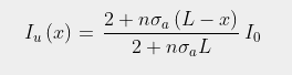
If we now apply the above results to a real system and consider the case of a column of gas of thickness L, and uniform density n that is independent of x, the model outlined above means that the upwelling radiation will vary with x through the gas as (see Post 88)

(91.8)

where I_o is the intensity of radiation entering the gas at x = 0, while the downwelling radiation will vary as

(91.9)

The difference between I_u(x) and I_d(x) will be constant (ΛI_o), as required by energy conservation, and will be equal to the amount transmitted at the end of the column (i.e. at x = L), so 

(91.10)

In Fig. 91.3 below I have suggested what I_u(x) and I_d(x) might look like through a 500 metre long horizontal column of air with 420 ppm of CO₂ when it is irradiated with 15 µm infra-red radiation from one end. It should be noted, though, that this theoretical data is based on an estimated value for the scattering cross-section of the CO₂ molecules that could be almost a factor of ten too small. Nevertheless, it still illustrates qualitatively how the transmission of 15µm infra-red radiation changes through the gas, and also how the Greenhouse Effect (as defined by the relative intensity of the reflected radiation at x = 0) is related to this transmission (see the red curve in Fig. 91.3).

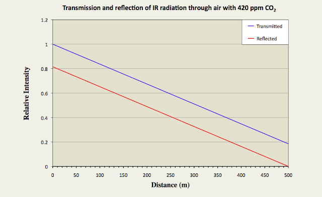
Fig. 91.3: The relative intensities of transmitted (I_u) and reflected (I_d) radiation along a 500 metre column of air containing 420 ppm of CO₂ with an absorption cross-section of 1.6 x 10^-24 m².

The graph in Fig. 91.3 suggests that a 500 metre column of air will transmit less than 18% of the incident radiation and reflect back the rest. The question is: is this more or less than that predicted by the Beer-Lambert law? The answer to this can be seen in Fig. 91.4 below.

Fig. 91.4: The relative intensities of radiation transmitted  through a column of air of length L containing 420 ppm of CO₂ with an absorption cross-section of 1.6 x 10^-24 m² based on two different models: (i) a backscattering model described by Eq. 91.10 (blue curve), and (ii) the Beer-Lambert law (red curve).

The blue curve in Fig. 91.4 demonstrates how the transmission through a column of air would decrease with the length of the column, L, if half of the absorbed radiation is backscattered or re-emitted in the reverse direction and half is re-emitted in the forward direction. The result is a curve that decays with L in accordance with Eq. 91.10. The red curve on the other hand shows how the transmission would change if it followed the (commonly accepted) Beer-Lambert law where the transmitted intensity varies with L as

(91.11)

What is clear is that the Beer-Lambert law underestimates the transmission for large values of L, and in effect predicts that there is no significant transmission beyond 400 metres. The blue curve shows that this is not the case with over 10% transmission for a column of length 1000 metres. In practice this means that the Beer-Lambert law will massively underestimate the impact of future increases in CO₂ levels because it will assume that the backscattering is already operating at close to 100% or saturation with 420 ppm of CO₂. Yet clearly it is not. In fact even at 10 km (the effective thickness of Earth's atmosphere) there is still more than 1% transmission. While this is small, it is not insignificant, particularly when considering the relatively small changes to the overall size of the Greenhouse Effect that are needed to create a warming of 1.5°C.

Caveats

The only condition I have applied to the proof and discussion described here is that set out in Eq. 91.4, which basically demands that each layer of the gas radiates the same amount of energy at each wavelength as it absorbs from the two fluxes, I_u(x) and I_d(x). This will be true provided all the heat of wavelength λ entering the gas originates from the Earth's surface at the bottom of Fig. 91.2, or at the very top of the atmosphere. In which case, the exact functional forms of I_u(x) and I_d(x) will depend only on the functional form of n(x) and the boundary conditions. However, at the top of the atmosphere this condition will not be satisfied as some of the incoming ultraviolet radiation from the Sun is absorbed there before it reaches the ground and so gets converted to infra-red radiation within the upper atmosphere. This means that Eq. 91.4 is no longer satisfied for each and every infra-red wavelength of interest within the gas.

In my next blog post I will consider a number of distinct and important examples to demonstrate how dependent the transmission is on the density profile of the gas, n(x), and also on the location of the heat source(s). These examples will also show that even when it sometimes looks like there is no Greenhouse Effect in operation, it is still there.

12. Black body radiation and Planck's law

Before you can understand how the Earth is heating up, you need to understand why it is warm in the first place. That means you need to appreciate the basic physics. Central to an understanding of how the Earth's surface temperature comes about are two important laws of physics: Planck's law and the Stefan-Boltzmann law. Both these laws describe in different ways how electromagnetic radiation is emitted from what in physics is termed a black body. Together they explain why the Earth's surface temperature is as it is.

Almost all the Earth's energy (other than a bit of geothermal energy, some naturally occurring nuclear decay, and a few cosmic rays) comes from the Sun. The Sun is predominantly a ball of fiery hydrogen plasma with a surface temperature of about 5505 °C (or 5778 K). The energy it produces comes from the nuclear fusion of that hydrogen into helium within its core (the core being defined as the region of the interior that is less than 0.7R_s from the centre, where R_s is the distance from the centre of the Sun to its outer edge). This fusion process gives off electromagnetic radiation with a range of frequencies, but which are mainly in the visible portion of the electromagnetic spectrum. It is the force of this radiation pushing out as it tries to escape that stops the Sun collapsing into a black hole under its own gravitational force. It also takes up to a year for many of these photons (particles) of light to actually escape. By contrast it only takes a further 8 minutes and 24 seconds for them to reach Earth.

The energy released by the Sun is 3.9 x 10²⁶ joules per second, or a power of P = 3.9 x 10²⁶ W. This is dispersed uniformly in all directions so that by the time it reaches Earth (at a distance r = 1.519 x 10¹¹ m from the Sun), it has spread out (due the inverse-square law) over a sphere in space of area A = 2.9 x 10²³ m² (= 4πr²). This means that the intensity of the radiation that we receive is P/A, or 1361 W/m². This is the power per unit area reaching Earth at the top of its atmosphere, and it still comprises the full range of different frequencies that were emitted from the Sun, each with a different relative intensity, as illustrated below in Fig. 12.1.

Fig. 12.1: The electromagnetic radiation output of the Sun (yellow) and the radiation received at ground-level on Earth (red).

What Fig. 12.1 shows is that the Sun's radiation output closely (but not exactly) resembles that from a black body of temperature 5250 °C (black curve), and that not all this radiation arrives at ground-level on Earth. Some is blocked by the atmosphere and reflected back into space.

In physics a black body is defined as an object that absorbs all the electromagnetic radiation that falls on its surface. It also has the property that when it is in thermal equilibrium with its surroundings at a constant thermodynamic temperature (i.e. the temperature measured on the kelvin scale), then it will emit heat in the form of electromagnetic radiation across a continuous range of frequencies. The distribution or spectrum of those frequencies is known as the black body spectrum, and it always has the normalized functional form shown in Fig. 12.2 below.

Fig. 12.2: The black body frequency spectrum.

The curve in Fig. 12.2 is described by the general equation

(12.1)

where a = 15/π⁴ is a scaling constant that ensures that the area under the curve is 1, and the parameter x depends on the thermodynamic temperature T (in kelvin) and the electromagnetic frequency (ν) as follows:

(12.2)

The other terms are Planck's constant, h, and the Boltzmann constant, k. By using the normalized variable x in Eq. 12.1 instead of ν and T, the equation can be applied universally. It is also worth noting that as λν = c, where λ is the wavelength of the radiation and c is the speed of light, it follows that x = b/Tλ where b = 14387.9 µm.K.

The actual intensity of the radiation emitted by a black body is then given by Planck's law as follows

(12.3)

where B(ν,T) represents the power per unit area of the surface emitted per steradian of solid angle. The total power emitted by a unit area of the surface, I(T), is therefore the sum of B(ν,T) over all frequencies and solid angles (this adds a factor of 2π for the half sphere the emission is flowing into).

(12.4)

We have already defined in Eq. 12.1 that

(12.5)

so it follows that

(12.6)

The result is known as the Stefan-Boltzmann law and σ = 5.67 x 10^-8 Wm^-2K^-4 is the Stefan-Boltzmann constant. This law represents the power that will be emitted from a perfect black body at a temperature T. This therefore represents the maximum power that any real object at that temperature can emit. In reality the emission is always less because no object behaves like a perfect black body, except a black hole.

What this demonstrates is that the power density output of a black body is not only proportional to the fourth power of the temperature, but it depends only on temperature. All the other quantities in σ are fundamental constants that cannot be changed. From this law we can therefore work out the maximum power output of the Sun. The surface temperature is 5778 K, so from Eq. 12.6 the power density of the emitted radiation is 63.2 MW/m². As the radius of the Sun is about 700,000 km, the surface area is 6.16 x 10¹⁸ m². So the total power output is 3.9 x 10²⁶ W, in agreement with the value at the top of this post.

Using these same equations we can now work out how hot the Earth will become when illuminated by the Sun's rays. We have already determined that the radiation intensity at the top of the atmosphere is I_TOA = 1361 W/m². The amount of power captured by the Earth will therefore be I_TOA multiplied by the cross-sectional area of the Earth πR_E² where R_E is the Earth's radius. But, as the Earth spins on its axis, this energy will need to heat up the entire surface area of the sphere, i.e. an area of 4πR_E². So the mean power density striking the Earth's surface will be a quarter of 1361 W/m², or 340.25 W/m².

This power will heat up the surface of the Earth until the point is reached where the temperature of the surface is high enough to ensure that the power that the Earth re-emits through the Stefan-Boltzmann law balances the incoming power from the Sun. This will happen when the surface temperature T_s is high enough so that σT_s⁴ = 340.25 W/m². This equates to a temperature of T_s = 278 K or 5 °C. This is not the mean temperature of planet Earth, though. It is what the mean temperature would be if the Earth had no atmosphere and the surface were completely absorbant and black. Except that this neglects the effects of the curvature of the Earth and its thermal conductivity. The former would mean the temperature at the poles would barely rise above 3 K (-270 °C), and that at the equator it could be as high as 393K or 120 °C in the daytime. The thermal conductivity of the surface would, on the other hand, mitigate these extremes.

In reality much of the incoming radiation is reflected by the atmosphere, the clouds, and the surface. This is the origin of the difference in the red and yellow areas in Fig. 12.1. The net result is that only about 161 W/m² gets absorbed by the Earth's surface, so according to Eq. 12.6 the surface temperature should not rise above 231 K, or -42 °C. However, this isn't true either. The mean temperature is actually closer to 289 K, or +16 °C. This is where the Greenhouse Effect comes into play.

While the atmosphere stops much of the incoming radiation getting in, it also stops much of the longer wavelength radiation emitted by the surface (and acting as a black body at 231K) getting out. Because the surface of the Earth is at a much lower temperature than the Sun, most of the radiation it emits will be at a much lower frequency, or longer wavelength. Some of this radiation then gets reflected back by the atmosphere, and in particular by the greenhouse gases, carbon dioxide and water vapour.

If the fraction reflected back we denote by f, and the reflected power is I_r, then it follows that I_r = f I_T, where I_T is the total power emitted from the surface. But as I_r is now incident on the Earth's surface, it too must be absorbed and add to the heating. It therefore follows that

(12.7)

where I_o = 161 W/m² is the original power absorbed by the Earth's surface. Following some elementary algebra we then obtain the result

(12.8)

As f is a number between 0 and 1.0, it follows that I_T will be greater than I_o. That in essence is the Greenhouse Effect with I_T being the power emitted from the Earth's surface with the Greenhouse Effect included, and I_o being the power emitted with it omitted. The only debate is what the value of f is, and by how much it is changing. Based on a surface temperature of 289 K, it would appear that f = 0.593; in other words 59.3% of the emitted power is reflected back. It is this value that I will look at in more detail next time when I discuss the Earth's energy budget.

On a final note, I will now go back to the emission spectra in Fig.12.1 and Fig. 12.2. There is an inconsistency here in that the first is a function of wavelength (λ), while the second (and most of the subsequent equations) is a function of frequency (ν). Does this matter? Well yes, particularly if you are wanting to calculate the total energy, or find the emission peak.

The peak or maximum of the curve in Fig. 12.2 occurs when x = 2.821, which means that for any object at a constant thermodynamic temperature, T, the frequency at which the maximum amount of radiation is emitted from that object, ν_max, is determined by the following formula:

(12.9)

For the Sun with a surface temperature of 5778 K, the peak frequency is 3.39 x 10¹⁴ Hz or 339 THz.

For those who may have forgotten their basic high-school physics, I remind you that frequency and wavelength are related by the equation λν = c, where c is the wave speed. For electromagnetic radiation c is the speed of light and it is always constant and the same for all wavelengths and frequencies. This means as the wavelength increases, the frequency decreases, and visa versa. It also means that as the speed of light is 3 x 10⁸ m/s, the frequency ν_max corresponds to a wavelength of 885 nm. Yet the peak in the solar spectrum in Fig. 12.1 is at 500 nm. So why are these two numbers not the same?

Well the crux of the problem is this. The theoretical black body spectrum in Fig. 12.2 with its peak at 2.821 in dimensionless units is a scaled version of Eq. 12.3. The quantity B(ν,T) represents the power density for each unit of frequency. When you integrate the area under the curve you get the total power. Now if you plot B(ν,T) as function of wavelength (λ) you are basically plotting the function below

(12.10)

For the case T = 5778 K this will still have a peak at λ = 885 nm, but when you integrate under this curve with respect to λ you do not get the result in Eq. 12.6. In other words, the area under this curve is not equal to the total power density. Instead you need to integrate with respect to the frequency and that means making the following transformation:

(12.11)

Note the switch of limits in Eq. 12.11 (zero to infinity and the reverse). The first switch occurs because the limits are now for λ and not ν. The second switch is because the differential of ν with respect to λ yields -c/λ² and removing the minus sign reverses the limits again. The result is that the equivalent spectral function for wavelength will be

(12.12)

If the function D(λ,T) is integrated over all wavelengths, the total power density is obtained.

(12.13)

Because the index of 1/λ in the function D(λ,T) is different from the index of ν in B(ν,T), it follows that the peaks in each spectra will be at different wavelengths because these are now inherently different equations. We can demonstrate this by defining a new dimensionless parameter y such that

(12.14)

where x is the same term as was introduced in Eq. 12.2. It then follows from Eq. 12.1, and using the differential result from Eq. 12.11, that we can define a second dimensionless term for λ that has the form

(12.15)

where again a = 15/π⁴. The area under this curve does indeed equal unity as before

(12.16)

which means that the function D(λ,T) can be rewritten to incorporate q(y) as follows:

(12.17)

If the function q(y) is plotted as a function of y, the result is the curve shown in Fig. 12.3 below.

Fig. 12.3: The black body wavelength spectrum.

The peak or maximum of the curve in Fig. 12.3 occurs when y = 0.201, which means that for any object at a constant thermodynamic temperature, T, the wavelength at which the maximum amount of radiation is emitted from that object, λ_max, is determined by the following formula:

(12.18)

This in turn leads to Wien's displacement law, which states that the product of the black body temperature, T, and the peak wavelength at that temperature, λ_max, is always equal to the same constant. In other words

(12.19)

The value of W_λ is 2.90 x 10^-3 Km. That means that when the temperature of the object is 5778 K, the peak wavelength will be 501 nm. This is why the peak of the solar spectrum in Fig. 12.1 is in the visible region of the spectrum corresponding to yellow light. Then, if the temperature decreases, so the peak wavelength will move to higher wavelengths as shown in Fig. 12.4 below.

Fig. 12.4: The black body wavelength spectrum at different temperatures.

However, it is not just the wavelength spectrum that obeys Wien's displacement law; the frequency spectrum does as well, it is just that the constant W_ν is different. Substituting c/λ_max for ν_max in Eq. 12.9 results in Eq. 12.20.

(12.20)

The value of W_ν is 5.11 x 10^-3 Km. This means that when the temperature of an object is 5778 K, the peak wavelength for its thermal emission will be at 884 nm. But while the position of the peak may change, what does not change is the amount of power found in a particular spectral range, even if that range appears at different places in Fig. 12.2 and Fig. 12.3.

For example, visible light is generally found between wavelengths of 400 nm and 800nm. In the case of the solar spectrum, the 400 nm radiation will have an equivalent x value of 6.236 according to Eq. 12.2 and a y value of 0.160 according to Eq. 12.14. For 800 nm radiation the values are x = 3.118 and y = 0.321. If the area under the curve in Fig. 12.2 between x = 3.118 and x = 6.236 is measured, it turns out to be 0.460 or 46.0% of the total area under the curve. If we do the same for the curve in Fig. 12.3 between y = 0.160 and y = 0.321 then we get the same result. Perhaps more interestingly, and relevant is, if you do the same for a 289 K spectrum for wavelengths between 13.89 μm and 16.13 μm you get an answer of 10.5%, but that is another story.