87. How the Greenhouse Effect on Earth changes with increasing carbon dioxide concentration

In my previous post (Post 86) I explained how infra-red photons emitted by the Earth's surface interact with carbon dioxide (CO₂) in the atmosphere to create the Greenhouse Effect. I also showed that increasing the temperature of the planet and increasing the concentration of carbon dioxide in the atmosphere will both lead to an increase in the width of the 15 µm absorption band of CO₂. This in turn will increase the amount of radiation that is backscattered by the CO₂, and therefore increase the amount of radiation heating the surface of the planet. 

In this post I will attempt to quantify the temperature increase for different increases in the CO₂ content of the atmosphere using the results presented in Post 86 and Post 85. What I will show is that the increase in atmospheric levels of CO₂ from 280 ppm in 1750 to almost 420 ppm today can only be responsible for at most a 0.5°C increase in average temperatures. This is only about 40% of the 1.2°C claimed by the IPCC and climate scientists. In fact the actual temperature rise due to CO₂ is likely to be less than half the calculated value of 0.5°C due to the masking effects of water vapour, and could be as little as 0.1°C. To put this into context, this is less than the values I have calculated for urban heating effects from waste heat (see Post 14 and Post 29) which would persist even without the use of fossil fuels.

The maths and physics

The starting point for this analysis is the quantum structure of the absorption band. This is shown in Fig. 87.1 below and was discussed in detail in Post 86. The key issue is the height of the various absorption lines in the P and R branches. These are identified by their angular momentum quantum number, J, which is numbered for each branch from the centre of the band, Q. 

Fig. 87.1: The detailed structure of the 15 µm absorption band for CO₂ showing the absorption peaks associated with rotational transitions.

In Post 86 I also showed that the width of the 15 µm band is determined by the value of J that satisfies the following equation (see also Eq.86.9), this value being denoted as J_th.

(87.1)

In this equation T is the thermodynamic temperature in kelvins, k is the Boltzmann constant, h is Planck's constant and B is the frequency of the rotational angular momentum states. For the rotational transitions shown for CO₂ in Fig. 87.1, hB = 0.1 meV and is equal to half the energy separation of the lines in the spectrum in Fig. 87.1. The other terms will be explained below.

 

The Z term

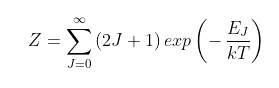
The term Z is a normalization term equal to the total number of possible rotational states per molecule in the R (or P) branch as follows. 

(87.2)

 

In the case of Earth where the mean surface temperature T = 289 K, the term Z = 249.3. The energy term E_J = J(J+1)hB. As the degeneracy term (2J + 1) is the differential of the J component of the energy term J(J+1), it follows that for large T the summation in Eq. 87.2 reduces to an integral over all J states, in which case Z ≈ kT/hB.

 

 

The N_o term

 

The term N_o in Eq. 87.1 is equal to the total number of CO₂ molecules per unit surface area found in the R branch. This can be estimated as being equal to approximately half the molecules, with the other half being in the P branch which is assumed to be the mirror image of the R branch (but is not really as was explained in Post 86). This also neglects the significant number of CO₂ molecules (particularly at low temperatures) found in the Q peak. Nevertheless, this approach does at least set an upper limit to the width of the R branch, and thus the width of the 15 µm band as a whole. And as will be shown below, it does give results that are remarkably accurate. As the number of CO₂ molecules per unit surface area found on Earth is 150 moles per square metre, it therefore follows that N_o is equal to 75 mol/m².

Calculating N_th and J_th.

The final remaining parameter to calculate is N_th. Ideally, if the absorption band edge had vertical edges, it would be the threshold number of CO₂ molecules per unit area that are just sufficient to completely block the radiation and would be equal to the reciprocal of the scattering cross-section, σ_s. As σ_s for CO₂ molecules is estimated to be between 10^-24 m² and 10^-23 m² in the 15 µm band, that would imply a value for N_th of about 1 mol/m². In practice, however, the band edge is curved so the usual definition of the edge is to take the position of the half maximum. This means using a value of N_th = 0.5 mol/m² is more appropriate.

With all the parameters now set we can calculate J_th using Eq. 87.1 above. The result we get is 29.4, which when multiplied by the line spacing, 2hB, gives the width of the R branch as 47.4 cm^-1 in wavenumbers. Assuming the P branch is identical means that the 15 µm band will extend from 619.6 cm^-1 to 714.4 cm^-1, or from 14.00 µm to 16.14 µm. This is remarkably close to the 14.2 µm to 16.2 µm that is generally observed for the peak in the absorption.

Having calculated the width of the 15 µm band with an atmospheric CO₂ concentration of 420 ppm, we can also repeat the procedure for any other CO₂ concentration of our choosing. For example, an atmospheric CO₂ concentration of 280 ppm that is characteristic of global conditions in 1750 leads to a value for J_th of 27.3, which means that the width of the R branch would be 44.0 cm^-1.

The temperature rise

In Post 85 I showed how the reflection of a fraction f of outgoing infra-red radiation would reheat the Earth's surface and cause the radiation it absorbed to increase from I_o to a higher value I_T as follows

(87.3)

Then in Post 86 I showed how the width of the 15 µm absorption band could be used to determine the value of f by calculating the relative area of this band under the absorption spectrum (see Fig. 86.1). This can then be used to infer a temperature rise due to the absorption by utilizing the Stefan-Boltzmann law,

 I = σT⁴. 

(87.4)

If I_T is the intensity of radiation emitted by the Earth's surface normally (i.e. 396 W/m²), and f is the fraction of radiation reflected back by the CO₂, then the intensity of radiation emitted by the Earth's surface without the CO₂ greenhouse effect will, according to Eq. 87.3, be I_o = (1-f)I_T. We can then use Eq. 87.4 to calculate the respective surface temperatures T_f and T_o for each radiation emission intensity, I_T and I_o. The difference in the two temperatures will be the warming due to the CO₂.

I showed above that an atmospheric CO₂ concentration of 420 ppm leads to an absorption band that extends from 14.00 µm to 16.14 µm. Combining this with the black body spectrum of the Earth at T_f = 289 K (see Fig. 87.2 below) allows us to determine f to be f = 10.0%. This in turn implies that I_o = 356.1 W/m² (where I_o is the radiation intensity without CO₂ feedback), and thus T_o = 281.52 K. So the temperature rise due to CO₂ is 7.48 K.

 

Fig. 87.2: The electromagnetic emission spectrum for the Earth's surface at a mean temperature of 289K (blue curve) together with the absorption profile due to CO₂ between 14.00 µm and 16.14 µm (red curve).

Now if we reverse this calculation but use an atmospheric CO₂ concentration of 280 ppm, we find that the absorption band now extends from 14.06 µm to 16.05 µm, so f = 9.28%. The value of I_o = 356.1 W/m² will be the same as before but the addition of a different amount of CO₂ will change I_T and T_f because f is different. The new values will be I_T = 392.6 W/m² and T_f = 288.46 K. So the temperature rise from CO₂ is now only 6.94 K. This implies that the temperature rise since 1750 due to the atmospheric CO₂ concentration increasing from 280 ppm to 420 ppm is only 0.54°C (i.e. 7.48°C - 6.94°C). 

If we repeat this process for other past or future (potentially) CO₂ concentrations we can calculate a theoretical temperature rise for each. This is shown in the graph in Fig. 87.3 below with the temperature changes all measured relative to the 1750 value when the atmospheric CO₂ concentration was 280 ppm.

 

Fig. 87.3: The theoretical effect of an increasing atmospheric CO₂ concentration on the contribution of CO₂ to global warming.

What Fig. 87.3 demonstrates is that the expected temperature increase from an increase in atmospheric CO₂ has a logarithmic dependence on the CO₂ concentration. However, the trend for concentrations between 280 ppm and 420 ppm is fairly linear and leads to a 0.5°C increase. Overall it appears that doubling the CO₂ concentration leads to about 1°C (or 1 K) of warming.

The interpretation of the data

While the logarithmic trend shown in Fig. 87.3 is in general agreement with climate models, the magnitude of the temperature changes are not. Whereas Fig. 87.3 suggests that 420 ppm of CO₂ leads to about 0.52°C of warming, the IPCC and climate science are claiming the rise is much greater at about 1.2°C. The difference, I suspect, is probably down to the impact of water vapour. Unfortunately, there are many ways that water vapour can impact the temperature trend.

The conventional view from climate scientists is that water vapour is a positive amplifier; the theory being that a warmer climate causes the amount of water vapour in the troposphere to increase, thus creating even more warming. As I pointed out in Post 86, the total feedback factor for infra-red radiation, f, is about 59%, while CO₂ alone can only account for about 18%, assuming that the 15 µm CO₂ absorption band width is measured at its half-maximum points from 13.35 µm to 17.35 µm. So the assumption is that water vapour is responsible for the rest, and that as its atmospheric concentration is dependent on the temperature, its concentration will increase as the level of CO₂ increases. So this will make the feedback, f, increase about three times faster than from CO₂ alone and so massively increase the temperature change to 1.2°C. The problem with this theory is that it ignores two major snags. 

First, the 15 µm CO₂ absorption band overlaps with the H₂O absorption band, as shown in Fig. 87.4 below. At the high wavelength edge of the 15 µm CO₂ band (17 µm) the water vapour will absorb almost 100% of the outgoing radiation while at the low wavelength edge (13 µm) it will absorb about 50%. This means that about 75% of any increase in the width of the 15 µm CO₂ absorption band will be masked from the outgoing radiation by the water vapour. In which case the temperature rise will only be 25% of the predicted value, or about 0.13°C.

 

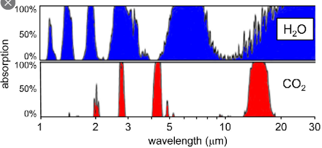
Fig. 87.4: The absorption bands of carbon dioxide and water vapour at sea level.

Secondly, the window in the H₂O absorption band extends from 8 µm to about 15 µm (using the half maxima points). This window allows only 41% of the Earth's outgoing infra-red radiation to escape. As we know that the feedback factor f = 59%, this means that water vapour could be responsible for absorbing and reflecting almost all the outgoing infra-red radiation that is absorbed and reflected. In other words, the 15 µm CO₂ band is not needed, and in fact is probably, largely redundant because it is hiding behind the water vapour. So again, a small change to the width of the CO₂ band is unlikely to cause any major temperature changes. This is why so many eminent physicists have so many serious reservations regarding the global warming predictions coming out of climate science.

 

The conclusions

1) Increasing the atmospheric CO₂ concentration will increase the width of its 15 µm absorption band.

2) In the absence of water vapour this could raise global temperatures, with an increase in CO₂ concentration from 280 ppm to 420 ppm resulting in a 0.5°C increase in global temperatures. 

3) The projected temperature increase has a logarithmic dependence on CO₂ concentration (see Fig. 87.3).

4) Water vapour masks most of the CO₂ 15 µm absorption band and so dominates the infra-red absorption. It can also account for almost all of the radiation feedback on its own.

5) The impact of water vapour means that an atmospheric CO₂ concentration rising from 280 ppm to 420 ppm could result in as little as a 0.13°C increase in global temperatures. This is ten times less than is currently claimed by climate science.

The caveats and discrepancies

In this analysis there are major uncertainties over the value of the CO₂ scattering cross-section, σ_s, and the widths of the CO₂ and H₂O absorption bands. This is also due to the difficulty in estimating the parameters N_o, N_th and J_th. However, the overall level of agreement between this analysis and real data and existing theory is encouraging.

The major discrepancy is between the measured width of the CO₂ 15 µm absorption band at its half maximum, where it extends from 13.35 µm to 17.35 µm, with the predicted width based on J_th where it extends from 14.00 µm to 16.14 µm. This difference could be due to line broadening from pressure broadening and temperature.

86. How photons interact with carbon dioxide molecules

In my previous post (Post 85) I countered a number of myths surrounding the greenhouse effect, and outlined how it really works. Many people falsely believe that it is caused by a heating of the atmosphere by outgoing infra-red radiation, but this is not the case. The key concept at the heart of the greenhouse effect is photon scattering, or more accurately, the absorption and re-emission of infra-red photons by molecules of the greenhouse gases. There are three main gases that perform this role: carbon dioxide (CO₂), water vapour (H₂O), and methane (CH₄). Each of these compounds absorbs electromagnetic radiation at its own set of unique wavelengths, but it is the absorption in the wavelength range between 6 µm and 90 µm that is key as this is where 96% of the thermal emission from the Earth's surface takes place. As CO₂ is seen as the most important player in terms of anthropogenic greenhouse gas emissions I will consider its role in greatest detail.

The emission and absorption spectra

In Fig. 85.1 of Post 85 I showed the main absorption bands of carbon dioxide in the infra-red part of the electromagnetic spectrum. In total there are four main bands at 2 µm, 2.7 µm, 4 µm and 15 µm, but only the 15 µm band is of any importance as the other three have energies that are way beyond the peak of the infra-red emission spectrum for Earth's outgoing radiation. This is illustrated in Fig. 86.1 below, where the blue curve represents the Earth's emission spectrum at 289 K and the red curve shows which frequencies are absorbed by CO₂. The area under the blue curve thus represents the total power of the radiation emitted at the Earth's surface, while the area under the red curve is the amount of radiated heat that can be absorbed and then reflected by CO₂.

 

Fig. 86.1: The electromagnetic emission spectrum for the Earth's surface at a mean temperature of 289K (blue curve) together with the absorption profile due to CO₂ between 14.2 µm and 16.2 µm (red curve).

The graph in Fig. 86.1 shows that only the 15 µm band is important as it is the only one close to the radiation peak. It is centred at 667 wavenumbers. Note: wavenumbers are the number of wavelengths of a radiation type that can fit in a distance of one centimetre. They are used because they are a measure of frequency, they result in much smaller numbers compared to other units of frequency like hertz, and are proportional to the photon energy of the radiation. The absorption bands at 2 µm, 2.7 µm and 4 µm correspond to wavenumbers of 5000, 3704 and 2500 cm^-1 respectively. Consequently, they can only interact with the tail of the frequency spectrum where there is very little energy being emitted (i.e. less than 1% of the total).

What the curves in Fig. 86.1 show is that only about 9% of the Earth's outgoing radiation can be absorbed and then reflected back by the carbon dioxide molecules in the atmosphere. In other words, the area under the red curve is only 9% of the area under the blue curve. Yet in Post 85 I showed that in reality 59% of the radiation is reflected back. The difference in these two numbers is largely due to water vapour which not only accounts for most of that difference (i.e. 50%), but also overlaps the 15 µm absorption peak of CO₂ (see Fig. 85.1 in Post 85), and so may render much of its function redundant. This is one reason why the claim that increasing the amount of CO₂ in the atmosphere will necessarily increase the strength of the greenhouse effect is disputed by many.

 

Fig. 86.2: The absorption bands of carbon dioxide and water vapour at sea level.

 

The other complicating factor is the actual width of the 15 µm band. The peak of maximum absorption generally stretches from about 14.2 µm to 16.2 µm, or from about 700 to 620 wavenumbers (or a width of 10.8 meV), and results in a feedback factor f = 9.2% and a temperature rise of 6.88°C. 

The band width, though, is dependent on both temperature and pressure. The full band at its tails can stretch from 12.5 µm to 18.5 µm (800 to 540 wavenumbers or a width of 32.2 meV), but absorption in the outer parts of the band decreases dramatically (see Fig. 86.2 above). If we were to use the full width of the band to determine the backscatter it would result in 26.8% of the outgoing radiation being reflected (see Fig. 86.3 below) and a temperature rise of 21.7°C; still much less than the 59% backscatter and the 58°C temperature rise that is actually seen.

Fig. 86.3: The electromagnetic emission spectrum for the Earth's surface at a mean temperature of 289K (blue curve) together with the potential absorption profile due to CO₂ between 12.5 µm and 18.5 µm (red curve).

A more realist estimate would be achieved by considering the width at the half maximum points of the band. This will be from about 13.35 µm to 17.35 µm (749 to 576 wavenumbers or a width of 21.4 meV) and would result in an absorption and reflection of 18.1%. This equates to a temperature rise at the surface of the Earth of 14.1°C.

Backscattering by Rayleigh scattering

The photons of infra-red radiation emitted by the Earth's surface interact with the carbon dioxide in two ways. One is by elastic scattering and the other via absorption and re-emission.

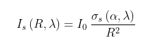
In elastic scattering the photons basically bounce off the CO₂ molecules like the collision of two billiard balls. This is the basis of what is known as Rayleigh scattering, named after the nineteenth-century British physicist Lord Rayleigh (John William Strutt), and it is a result of the electromagnetic interaction of the photon with the charged particles (electrons and protons) in the molecule. After collision the photons will end up travelling in a different direction. Some will be reflected back while others will carry on in a forward direction. It is the ones that are reflected that contribute to the greenhouse effect. The intensity of photons at a distance R from the molecule after being scattered through an angle θ is given by the equation

(86.1)

It can be seen that the overall scattering probability depends on the wavelength of the radiation (λ) and the strength of the polarizability of the molecule doing the scattering (α). The strong inverse dependence on wavelength explains why the sky is blue in daylight. This happens because blue light photons with wavelengths of about 400 nm scatter sixteen times more often as they travel through the Earth's atmosphere than red light photons of wavelength 800 nm do. It also means that Rayleigh scattering from carbon dioxide at wavelengths of 15 µm is about a billion times less likely to occur than the scattering of visible light. This is because the wavelengths of the photons being scattered are at least twenty times greater, so the scattering rate of 15 µm photons by CO₂ molecules is at least 160,000 times less than for visible light. But in addition, the proportion of CO₂ in the atmosphere is only 0.042% of all the molecules. This equates to about 150 moles of CO₂ per square metre of the Earth's surface.

Another way of describing the strength of the scattering is via a scattering cross-section, σ_s. This is a measure of the effective cross-sectional area of each molecule that a photon will see, or alternatively how effective that molecule is at blocking the radiation. The scattering cross-section is usually (but not always) much less than the physical dimension of the molecule. 

Using the definition of scattering cross-section Eq. 86.1 becomes

(86.2) 

 

where the scattering cross-section, σ_s(λ,α) is a function of both the wavelength of the radiation (λ) and the polarizabilty (α) as follows

(86.3)

All molecules have their own unique polarizabilities; a list of some of the more common ones can be found here. Most of the common atmospheric gases have similar values for α, although the value for CO₂ is about 50% higher than most. So scattering from CO₂ is about twice that from oxygen and nitrogen. Nevertheless, this still means that with only about one in a billion 15µm photons being scattered by the 150 moles per square metre of CO₂, the Rayleigh scattering cross-section of CO₂ at this wavelength equates to only about 10^-35 m². This is a million billion times smaller than the actual size of the molecule.

The key point, therefore, is that Rayleigh scattering is of negligible importance when discussing the greenhouse effect because it is a billion times weaker than the Rayleigh scattering we see of visible light. Absorption and re-emission of photons by the 15 µm band are the more important processes, but as I will explain next, their combined behaviour in terms of scattering is very similar to Rayleigh scattering, but much stronger.

Backscattering by absorption and re-emission

Almost all backscattering by carbon dioxide occurs via a process of absorption and re-emission of the infra-red photons with wavelengths in the region of the 15 µm band (i.e. 12.5-18.5 µm). The closer these photons are in wavelength to the centre of the band the more strongly they are absorbed.

Once excited, the molecule may then collide with other molecules and exchange its extra energy with them, thereby heating the gas as a whole. But once all the gas is heated equally, thermal equilibrium will be established where some of the excited CO₂ molecules will re-emit photons at the same rate that other CO₂ molecules are absorbing them. This situation physicists refer to as the steady state. At this point, for every photon being absorbed, another is being re-emitted by another molecule in a random direction.

Ultimately, every molecule wants to get to its lowest energy state, so while bombarding it with radiation will force its energy state to increase, it also increases the rate at which it tries to lose energy. So eventually an equilibrium is achieved where the amount of radiation being absorbed by the gas balances the amount that is lost through re-emission. The key point to note, though, is that the re-emission is a random process that can result in the emitted photons being ejected in any direction. In contrast, most of the absorbed photons come from a single direction: the Earth's surface. This means that fewer of the re-emitted photons end up travelling away from the surface as some are reflected back. Those photons that are reflected back then provide additional heat to the surface, thereby raising its temperature even further. This is the origin of the Greenhouse Effect. 

 

Structure of the absorption band

The infra-red photons emitted from the Earth's surface are absorbed by carbon dioxide via a process of molecular excitation where the molecule is promoted to a higher energy state. Usually this process is in the form of electrons within the molecule moving to higher energy levels, but those transitions are usually of very high energy (several electron volts or eV) and so they only result from the absorption of visible or ultraviolet light. 

The 15 µm transition in carbon dioxide is in the infra-red part of the spectrum and so it is of a much lower energy (about 83 meV). Instead it results from a bond stretching excitation where the molecule bends, as shown in mode v₂ in Fig. 86.4 below, under the action of the incoming electromagnetic wave of the photon. This bond stretching occurs because of an uneven distribution of electric charge within the molecule which then interacts with the electric field of the incoming electromagnetic wave or photon.

Fig. 86.4: The three vibrational modes of carbon dioxide. The symmetric stretch mode (v₁) occurs at 7.5 µm but does not absorb because of symmetry violation. The bend mode (v₂) corresponds to absorption at 15 µm, while the asymmetric stretch mode (v₃) corresponds to absorption at 4.3 µm.

In addition to the bond stretching, a much smaller amount of energy from the incoming photon may go towards increasing the angular momentum or rotational spin of the molecule. This leads to "wings" or branches to the central band as shown in Fig. 86.5 below, with the lower energy branch being denoted as the P branch, and the higher energy one the R branch. It is these branches that cause the band to broaden from a single sharp peak Q at 15 µm to a broader band stretching from 12.5 µm to 18.5 µm.

 

Fig. 86.5: The detailed structure of the 15 µm absorption band for CO₂ showing the absorption peaks associated with rotational transitions.

 

The branches P and R are each comprised of a set of evenly spaced discrete transitions, each one matched to a different change in rotational energy of the molecule due to a change in its angular momentum state J by an amount ∆J = ±1. This is because the incoming photon has an angular momentum quantum of J = +1 and angular momentum must be conserved in the absorption process. The R branch arises from absorption processes where the photon causes the molecule to spin faster, while the P branch arises from absorption processes where the photon causes the molecule to spin more slowly (i.e. the angular momentum of the photon is in the opposite direction to that of the molecule). The two branches are, in theory, mirror images of each other, but in practice centrifugal distortion and rotational-vibrational coupling lead to the line spacing increasing at lower energies.

As the energy of each rotational state J of the molecule is (ideally) equal to J(J+1)hB where h is Planck's constant and B is given by

(86.4)

with I being the moment of inertia of the molecule about its spin axis, the energy change associated with a transition from state J to J+1 when a photon is absorbed will be ±2hB(J+1) (see here). So the absorption peaks due to changes in rotation have an ideal energy separation of 2hB, or about 1.54 wavenumbers (cm^-1) or 0.2 meV for lines in the 15 µm band of carbon dioxide. 

These individual line transitions are also broadened via doppler broadening due to the different speeds and directions of motion of the various molecules, and pressure broadening due to collisions with other molecules in the atmosphere. Both of these broadening mechanisms are temperature dependent and increase as the temperature increases. The result is that the width and overall scattering cross-section of each line will increase with temperature thereby narrowing or closing completely the gaps between the individual rotational lines in the spectrum. For lines in the 15 µm absorption band of CO2 the typical scattering cross-section is about 10^-23 m², which is about one trillion (i.e. 10¹²) times greater than the scattering cross-section of each molecule due to Rayleigh scattering at the same wavelength.

In addition, an increase in temperature will shift the position of the peak or maximum in both the P and R branches, J_max (again see here). This is because the height of each line in the 15 µm band is dependent on both its J number and the temperature. Each line has a degeneracy of 2J+1, while the probability of exciting that rotational J mode depends exponentially on both energy and temperature. This means that the relative occupancy of each mode, N_J, is given by 

(86.5)

where the energy E_J of the mode J is given by J(J+1)hB, N_o is the total number of excited modes, and Z is a normalization term that is equal to the sum of the probabilities.

 (86.6)

This also explains why the P and R branches in Fig. 86.5 have peaks in their distributions. The occupancy of each rotational state N_J increases linearly with J via the degeneracy term 2J+1, but for large J decreases more rapidly due to the energy term E_J in the exponential. This leads to a maximum in the distribution, the position of which relative to the band centre at Q can be determined by differentiation with respect to J. The result is given by 

(86.7)

What this shows is that as the temperature of the gas increases, the position of the maxima will move further from the band centre at Q, so the overall width of the band will increase with temperature as well. This is because higher temperatures will lead to a higher proportion of CO₂ molecules in higher energy rotational states with larger J values. Generally, though, it takes a large temperature change to significantly widen the band. As the position of the R branch maximum relative to Q increases with temperature T as √T, it is reasonable to expect the width of the band to do the same.

Finally, if the width of the absorption band can change with temperature, then it can also change with CO₂ concentration. In this case the width will be set by the highest value of J for which N_J exceeds some threshold value N_th, this being the number of modes required to almost completely absorb the outgoing radiation at that wavelength. According to Eq. 86.5 this will be the value of J such that

(86.8)

Rearranging Eq. 86.8 gives the following result for the threshold J value, J_th, that defines the edge of the band

(86.9)

So Eq. 86.9 not only confirms that the band width varies approximately as √T, but also that it varies approximately as √ln(N_o). 

Conclusions

The dominant mechanism by which CO₂ molecules scatter infra-red radiation in the 15 µm band is by absorption and re-emission.

The absorption and re-emission process has a similar effect to that of Rayleigh scattering, but it is almost a trillion (i.e. 10¹²) times stronger. 

The width of the 15 µm band increases with temperature as √T, but increases much more slowly with CO₂ concentration (see Eq. 86.9).