75. Southern Asia - overall temperature trend STABLE to 1975

In my previous four blog posts I determined the temperature trends for India, Pakistan, Sri Lanka and Bangladesh using unadjusted temperature data. The number of stations used to calculate the mean temperature each month is shown in Fig. 75.1 below. In the first three cases no warming was detectable before 1975, and only a modest temperature increase of about 0.6°C thereafter. In the case of Bangladesh there was a continuous warming that amounted to less than 0.3°C. This is significantly different from the conventional narrative on global warming, and highlights the impact that temperature adjustments have on the warming trends published by most of the main climate groups. In almost all cases the affect of these adjustments is to increase the rate of warming in the final trend as most of the regional trends I have published on this blog have also illustrated. In this post I will combine the results for India, Pakistan, Sri Lanka and Bangladesh into a temperature trend for the region.

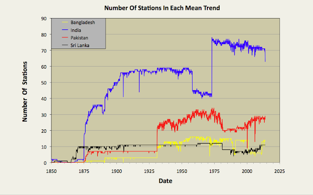
Fig. 75.1: The number of station records included each month in the mean temperature anomaly for each of four countries in South Asia.

In Post 70 I performed a similar task for data from the different countries in South-East Asia using two separate methods. One method just involved a simple average of temperature anomalies from all the different stations in the region, while the second used a weighting process that was used to average the mean anomalies for the different countries based on their land areas. If all the countries have similar densities of stations, then both methods should yield the same result. In the case of South-East Asia that was broadly the case for most countries other than Burma, but the differences in the two methods still led to a difference in the temperature trend gradients of almost 0.1°C per century. In the case of South Asia there are large differences in station density between countries, and these differences can also change over time, as shown in Fig. 75.2 below. For this reason, in this post I have chosen to adopt the area weighted method to determine the regional temperature trend.

Fig. 75.2: The station density each month for each of four countries in South Asia.

By comparing Fig. 75.1 and Fig. 75.2 it can be seen that India clearly has the most sets of station data, but it is Sri Lanka that has the highest density of stations. However, the temperature anomaly for Sri Lanka will also be subject to greater uncertainty as it is based on only a handful of stations (eleven at most). Then again, the contribution of the Sri Lanka stations to the final regional trend will be small due to the much smaller area of Sri Lanka compared to both India and Pakistan.

Fig. 75.3: The temperature trend for South Asia based on an average of anomalies from all long and medium stations. The best fit is applied to the monthly mean data from 1876 to 1975 and has a positive gradient of +0.19 ± 0.06 °C per century. The monthly temperature changes are defined relative to the 1951-1980 monthly averages.

Applying an area weighted approach to the calculation results in the temperature anomaly time series shown in Fig. 75.3 above. This is calculated by multiplying the mean anomaly data for each country (e.g. the monthly data in Fig. 74.2 for Bangladesh) by the area of that country, and then summing the resulting products for all four countries in the region. Then the result is divided by the total area of the four countries.

Like the equivalent anomaly time series for the individual countries, the regional anomaly exhibits very little warming before 1975 with about 0.5°C of warming occurring thereafter (see Fig. 75.3). To reiterate, this is the result that we get when we use the actual raw unadjusted temperature data for each station and not the adjusted/homogenized data that is generally favoured by climate scientists.

Fig. 75.4: Temperature trends for South Asia based on an average of Berkeley Earth adjusted data from all long and medium stations. The best fit linear trend line (in red) is for the period 1876-2005 and has a gradient of +0.66 ± 0.02°C/century.

If, however, we perform the same calculation with adjusted data (which is available in the same data file as the unadjusted data on the Berkeley Earth site) we get a quite different result as is shown in Fig. 75.4 above. There is now a strong and continuous warming trend from 1875 onwards. The total warming is claimed to be 1.25°C, with 0.5°C of this occurring before 1975 (see 10-year average in Fig. 75.4). This is still less than that claimed by Berkeley Earth and shown in Fig. 75.5 below. However, this is likely to be because Berkeley Earth included both Iran and Afghanistan in the Southern Asia region, and according to Berkeley Earth the regional temperature trends for both Iran and Afghanistan exhibit over 1.5°C of warming after 1970. That would help to explain the larger temperature rise post-1970 seen in Fig. 75.5 (almost 1°C) than is seen in Fig. 75.4 (only 0.7°C). What is harder to explain is why there is so much warming before 1900 in Fig. 75.5 when there is a) so little data with almost all being due to one or two stations in India, and b) very little increase in atmospheric carbon dioxide levels to cause such a temperature increase.

Fig. 75.5: The temperature trend for South Asia since 1790 according to Berkeley Earth.

Finally, if we compare the temperature trends for the four countries of South Asia we see that while there are broad similarities in their general trends over timescales of decades, there is only moderate correlation of more short term features and fluctuations (see fig. 75.6 below). The main reason for this is distance. The principal cities of Bangladesh (Dhaka), Sri Lanka (Colombo) and Pakistan (Karachi) are all at least 2000 km apart. As I demonstrated in Post 11, temperature anomaly time series from stations that are more than 1500 km apart are very poorly correlated as Fig. 11.2(a) in that post illustrates.

Fig. 75.6: A comparison of the temperature trends of Bangladesh, Pakistan and Sri Lanka with that of neighbour India. For clarity the trends for Pakistan and Bangladesh are offset by +1°C and -1°C respectively.

Summary

The temperature trend for Southern Asia shows no warming before 1975 and only about 0.5°C thereafter (see Fig. 75.3).

The trend based on Berkeley Earth adjusted data shows significantly more warming (about 1.1°C in total), including significant warming (about 0.5°C) before 1975 (see Fig. 75.4).

74. Bangladesh - temperature trends WARMING 0.3°C

Despite being surrounded by India on threes sides, Bangladesh has a slightly different temperature trend to its larger neighbour. This may be because of a reduction in reliable data after 1999 where, in the case of India, the temperature rises abruptly by about 0.6°C; in the case of Bangladesh it does not. Between 1930 and 1990 where Bangladesh has the majority of its temperature data, the agreement with India is actually quite good.

 

Fig. 74.1: The (approximate) locations of the long and medium temperature records in Bangladesh. Those stations with a high warming trend between 1921 and 2010 are marked in red while those with cooling or stable trends are marked in blue. Those denoted with squares are long stations with over 1200 months of data.

 

Overall there are 17 temperature records for Bangladesh that have over 480 months of data (for full list see here). Of these three are long stations with over 1200 months of data, while the remainder are medium stations. In fact all the medium stations have at least 600 months of data. The locations of these stations are shown in Fig. 74.1 above. Their geographical spread is fairly even, which suggests that any simple average of their temperature anomalies should yield a fairly accurate approximation to the true mean temperature anomaly for the region. It can also be seen that over half of the stations have stable or cooling trends for the 90 years up to the end of 2010. 

Just as for my previous regional analyses, the monthly temperature anomalies for each station were calculated by subtracting the monthly reference temperature (MRT) for the relevant month from the unadjusted mean temperature for that month. These anomalies from the various long and medium records were then averaged to determine the mean temperature trend for the region. The resulting mean monthly temperature anomaly is shown in Fig. 74.2 below.

 

Fig. 74.2: The temperature trend for Bangladesh based on an average of anomalies from all long and medium stations. The best fit is applied to the monthly mean data from 1921 to 2010 and has a positive gradient of +0.27 ± 0.08 °C per century. The monthly temperature changes are defined relative to the 1931-1960 monthly averages.

 

The MRTs are different and specific to each station, but were always calculated using data from the same time period (in this case 1931-1960) for each station using the method described previously in Post 47. This ensures that the baseline reference temperature for each station is consistent so that all temperature changes over time are measured relative to the same point in time. However, no choice of 30-year MRT interval would have enabled all 17 station records to be included in the mean temperature in Fig. 74.2. This is because one station Berhampore (Berkeley Earth ID: 5388) has no data after 1957, while two stations, Dacca Tejgaon (Berkeley Earth ID: 152645) and Sylhet (Berkeley Earth ID: 152652), have virtually no data before 1956. An MRT interval of 1931-1960 allowed Berhampore to be included, thus increasing the number of stations with data before 1930 from three to four (see Fig. 74.3 below).I decided this was more beneficial in terms of overall data quality than having an extra two sets of station data after 1957.

Fig. 74.3: The number of station records included each month in the mean temperature trend for Bangladesh in Fig. 74.2.

 

The mean temperature trend for Bangladesh shown in Fig. 74.2 exhibits a slight warming of about 0.25°C after 1920. Yet the official Berkeley Earth trend suggests the warming is much greater, being almost 1°C after 1920 and nearly 1.5°C since 1830 (see Fig. 74.4 below). This is despite the fact that there is no real temperature data before 1875. So which data trend is correct?

 

Fig. 74.4: The temperature trend for Bangladesh since 1800 according to Berkeley Earth.

 

Well, if we average the Berkeley Earth adjusted data from all 15 stations used in this analysis (the adjusted data is listed on the Berkeley Earth site along with the raw data) we obtain trends that are very similar to those in Fig. 74.4 as the data in Fig. 74.5 below shows. This demonstrates two points. Firstly, it provides strong evidence that the averaging method we use to combine anomalies from the different stations is sufficiently accurate to avoid the need to use gridding and homogenization techniques. If this were not true then the data in Fig. 74.4 and Fig. 74.5 would not agree so well, but the uniform geographical distribution of stations across Bangladesh clearly facilitates this. But secondly, it shows that most of the warming presented in Fig. 74.4 comes from adjustments made to the data, and not from the raw data itself, otherwise the data in Fig. 74.5 would agree with the data in Fig. 74.2.

 

Fig. 74.5: Temperature trends for Bangladesh based on the average of anomalies for all long and medium stations using Berkeley Earth adjusted data. The best fit linear trend line (in red) is for the period 1921-2010 and has a gradient of +0.74 ± 0.03°C/century.

 

Finally, comparing the adjusted data in Fig. 74.5 with the unadjusted data in Fig. 74.2 allows us to quantify the contribution made to the trends in Fig. 74.4 by the Berkeley Earth data adjustments. These net adjustments are shown below in Fig. 74.6.

 

Fig. 74.6: The contribution of Berkeley Earth (BE) adjustments to the anomaly data in Fig. 74.5 after smoothing with a 12-month moving average. The blue curve represents the total BE adjustments including those from homogenization. The linear best fit (red line) to these adjustments for the period 1921-2010 has a positive gradient of +0.431 ± 0.014 °C per century. The orange curve shows the contribution just from breakpoint adjustments.

 

The data in Fig. 74.6 indicate that the adjustments made to the data by Berkeley Earth add at least 0.4°C of warming to the overall temperature trend after 1930. This explains why Fig. 74.4 and Fig. 74.2 appear so different.

 

Summary

It is clear from the temperature trend calculated using the raw data (see Fig. 74.2) that there has been no significant climate change in Bangladesh over the last 80 years. The long term temperature rise of 0.24°C is much less than the observed natural variation in the mean temperature.

The small temperature rise of 0.24°C since 1920 could be due to increased greenhouse gas emissions globally. Carbon dioxide levels in the atmosphere have increased from 307 ppm in 1930 to nearly 420 ppm today. But this temperature rise is much less than what mainstream climate science claims should be the case for this magnitude of change in CO₂.

Addendum

The regional average in Fig. 74.2 was calculated using 15 of the 17 possible sets of station data because of the choice of MRT interval. The stations at Dacca Tejgaon (Berkeley Earth ID: 152645) and Sylhet (Berkeley Earth ID: 152652) were excluded so that the station with much earlier data at Berhampore (Berkeley Earth ID: 5388) could be included. If the MRT interval is instead chosen to be 1951-1980 the reverse occurs with only Berhampore being excluded. The resulting mean temperature trend is shown below in Fig. 74.7. It has a slightly higher warming trend, but is otherwise very similar to Fig. 74.2.

Fig. 74.7: The temperature trend for Bangladesh based on an average of anomalies from all long and medium stations. The best fit is applied to the monthly mean data from 1921 to 2010 and has a positive gradient of +0.31 ± 0.08 °C per century. The monthly temperature changes are defined relative to the 1951-1980 monthly averages.