Monday, December 6, 2021

84. Southern Africa - a summary of temperature trends

Over the last fifteen months I have analysed the temperature data for nine different countries in southern Africa and calculated their temperature trends. My analysis began in September 2020 with South Africa (Post 37) before continuing on to Botswana (Post 38) and Namibia (Post 39) in October. More recently I have examined the temperature records of Madagascar (Post 77), Mozambique (Post 78), Zimbabwe (Post 79), Zambia and Malawi (Post 81), and Angola (Post 82).

The one constant for all these countries is the temperature trend since 1980. In almost all cases the climate shows evidence of warming, with the temperature rise varying between 0.5°C and 1.5°C. Before 1980 the picture is different with little or no temperature rise being seen, and in many cases (e.g. Madagascar, Zimbabwe, Zambia and Malawi) a significant cooling taking place. These results are summarized in the graphs below.

The main conclusions to be drawn here are as follows.

  • All the warming in southern Africa has occurred since 1980.
  • There is probably no warming before 1980, and possibly some cooling.
  • The net warming since 1850 is likely to be between 0.5°C and 1.0°C. This is less than the IPCC global value of 1.3°C, and much less than the land-based Berkeley Earth average of almost 2.0°C (see Fig. 80.1 in Post 80).

In the New Year I will return to the African data and analyse the data from countries in sub-Saharan and equitorial countries. In the meantime I will return to considering the physics of the Greenhouse Effect that I introduced in Post 12 (black-body radiation) and Post 13 (Earth's energy budget). In particular I will look to answer two questions: why is Venus so hot, and why is Mars so cold?


Fig. 37.2: The mean temperature anomaly (MTA) for South Africa since 1840. The best fit is applied to the interval 1857-1976 and has a gradient of +0.017 ± 0.056 °C per century. The monthly temperature changes are relative to the 1961-1990 monthly averages.


Fig. 38.3: The mean temperature anomaly (MTA) for Botswana since 1917. The best fit is applied to the interval 1917-1976 and has a positive gradient of +0.72 ± 0.26 °C per century. The monthly temperature changes are defined relative to the 1961-1990 monthly averages.


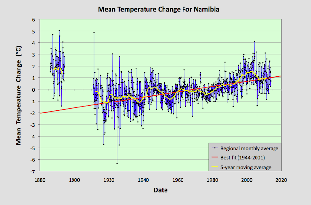
Fig. 39.8: The mean temperature anomaly (MTA) for Namibia since 1885. The best fit is applied to the interval 1944-2001 and has a positive gradient of +2.28 ± 0.17 °C per century. The monthly temperature changes are defined relative to the 1971-1990 monthly averages.


Fig. 77.6: The mean temperature anomaly (MTA) for Madagascar. The best fit is applied to the monthly mean data from 1932 to 2011 and has a negative gradient of -0.15 ± 0.07 °C per century.


Fig. 78.6: The mean temperature anomaly (MTA) relative to the 1931-1960 monthly averages for stations in Mozambique with over 300 months of data but excluding Lourenço Marques. The best fit is applied to the monthly mean data from 1921 to 1980 and has a positive gradient of +0.16 ± 0.12 °C per century.


Fig. 79.2: The mean temperature anomaly (MTA) for Zimbabwe relative to the 1971-2000 monthly averages based on an average of anomalies from stations with over 360 months of data. The best fit is applied to the monthly mean data from 1916 to 1975 and has a negative gradient of -0.96 ± 0.20 °C per century.


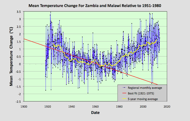
Fig. 81.2: The mean temperature anomaly (MTA) relative to the 1951-1980 monthly averages based on an average of anomalies from stations with over 360 months of data. The best fit is applied to the monthly mean data from 1921 to 1975 and has a negative gradient of -2.72 ± 0.17 °C per century.


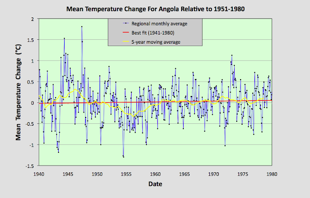
Fig. 82.5: The mean temperature anomaly (MTA) for Angola relative to the 1951-1980 monthly averages based on an average of anomalies from stations with over 300 months of data. The best fit is applied to the monthly mean data from 1941 to 1980 and has a positive gradient of 0.18 ± 0.17 °C per century.


Sunday, December 5, 2021

83. Is the BBC biased on climate change?

I am sure that for many people the answer to this question is obvious, and I suspect the answer depends on how strongly you believe in climate change. But consider this.

On the 25th August 2021 the BBC ran a story on their website reported on a UN claim that Madagascar was "on the brink of climate change-induced famine".


Well, it turns out that not everyone agrees. Because on the 2nd December 2021 the BBC reported that another group of scientists had cast doubt on the UN claim.


The issue I have with these two reports is that they do not appear to have been given the same prominence or weight on the BBC site. While the first gets its own webpage, the second seems only to get a small note on the BBC climate page list of recent updates (unless I have missed something), and certainly does not link to a full webpage article (although it does link to the original article). So having created a sensational climate change headline, the BBC then seems to have (partially) buried the opposing viewpoint, or rejection of it, which just happens to go against the prevailing narrative that most environmental disasters are now due to climate change. 

Personally, I strongly support the BBC and see it as an important part of the British media, one that is essential in protecting political diversity and democracy in the UK. I just wish it would be more objective and critical, rather than trying to be sensationalist, populist, mainstream and worst of all, "impartial". 

For reference, the actual climate change in Madagascar is shown below (see also Post 77).


Fig. 77.6: The mean temperature anomaly (MTA) for Madagascar. The best fit is applied to the monthly mean data from 1932 to 2011 and has a negative gradient of -0.15 ± 0.07 °C per century.


Tuesday, November 30, 2021

82. Angola - temperature trends STABLE

The biggest problem we are confronted with when it comes to determining the extent of climate change in Angola is a lack of temperature data. There is only one long station with over 1200 months of data and another four medium stations with over 480 months of data. Only two stations have a significant quantity of data before 1939, and they are both in the capital Luanda; and none have any reliable data after 1980 due to the protracted civil war. A full list of stations for Angola can be found here.

If we include stations with over 240 months of data, then there are a total of eighteen temperature records that we can use. Their locations are indicated on the map below in Fig. 82.1. Overall they are fairly evenly distributed across the country, although the stations with the longest temperature records are generally found nearest the coast. The consequence of this deficit of data is that it is impossible to definitively determine the temperature trend for the country either before 1940, or after 1980. Between 1940 and 1980 the data suggests that no warming took place.


Fig. 82.1: The (approximate) locations of the main weather stations in Angola. Those stations with a high warming trend between 1901 and 2000 are marked in red while those with a cooling or stable trend are marked in blue.


The monthly anomalies for each station were created in the usual manner, as outlined in Post 47. First a suitable thirty year interval was chosen for calculating the monthly reference temperatures (MRTs). In this case the period 1951-1980 was chosen as that corresponded to the interval that overlapped with the maximum number of station records. The twelve MRTs for each station dataset were calculated for each of the twelve months by averaging the monthly temperatures in the reference period for that station. The MRTs were then subtracted from all the respective monthly temperature data for that station to generate the anomalies. The anomalies from all the stations were then averaged to give the mean temperature anomaly (MTA) for the region in that month. Employing a simple average of the station data rather than using Kriging, homogenization and gridding is sufficiently accurate if the stations are fair evenly distributed, which the map in Fig. 82.1 suggests to be the case. The resulting mean temperature anomaly since 1875 is shown below in Fig. 82.2.


Fig. 82.2: The mean temperature anomaly (MTA) for Angola relative to the 1951-1980 monthly averages based on an average of anomalies from stations with over 300 months of data. The best fit is applied to the monthly mean data from 1881 to 1980 and has a positive gradient of 1.39 ± 0.08 °C per century.


The MTA in Fig. 82.2 exhibits a similar warming profile to the IPCC global trends, but this is somewhat misleading. The data before 1939 is based on only two stations, and both of these are situated in the capital Luanda (Berkeley Earth ID 151475 and 2824), while the data after 1980 is highly sporadic and discontinuous for all stations with data in this period. This is illustrated in Fig. 82.3 below which shows the station frequency count in the MTA in Fig. 82.2. 


Fig. 82.3: The number of station records included each month in the mean temperature anomaly (MTA) trend in Fig. 82.2.


The station with the longest data set is Luanda (Berkeley Earth ID 151475), the monthly anomalies of which are shown in Fig. 82.4 below. The second station in Luanda (Berkeley Earth ID 2824) has no data after 1973, while its data after 1951 is virtually identical to that of station 151475. Before 1951, however, the data from the two stations disagree by an average of almost 0.5°C. This hints that the two sets of station data may not be completely independent, or may be the result of combining other datasets.


Fig. 82.4: The temperature anomaly for Luanda relative to the 1951-1980 monthly averages. The best fit is applied to all the monthly mean data and has a positive gradient of 1.63 ± 0.06 °C per century.


The main conclusion to be drawn from Fig. 82.3 is that both the data before 1939 and the data after 1980 are unreliable. The data after 1980 is unreliable because there is so little of it, and it is highly fragmented. The data before 1939 is unreliable because it is based on just two stations that are located in the most highly populated region of the country. While these two stations do corroborate each other, particularly after 1951, they are still unlikely to be representative of the climate of the country as a whole. We know this because we see it in many countries and regions: strong warming in the major cities like Jakarta (see Post 31), Sydney (BE-151986) in NSW (Post 18) and Melbourne (BE-151813) in Victoria (Post 19), but a totally different temperature trend in the surrounding region.


Fig. 82.5: The mean temperature anomaly (MTA) for Angola relative to the 1951-1980 monthly averages based on an average of anomalies from stations with over 300 months of data. The best fit is applied to the monthly mean data from 1941 to 1980 and has a positive gradient of 0.18 ± 0.17 °C per century.


If we therefore just look at the data from 1940 to 1980 we see that there is no significant warming (see Fig. 82.5 above). The slight rise in the best fit line is at least five times less than the standard deviation of the MTA, and is almost the same as the uncertainty in the best fit. And this is also similar to the extent of the warming claimed by Berkeley Earth for this period (see Fig. 82.6 below).


Fig. 82.6: The temperature trend for Angola since 1840 according to Berkeley Earth.


However, the temperature trend for Angola according to Berkeley Earth (BE) does exhibit strong warming both before 1939 and after 1980. While the latter is certainly a reasonable assumption based on trends elsewhere in the region, it is not a conclusion that can be confidently presented based on the available data. As for the data in Fig. 82.6 before 1939, this may be supported by the station data from Luanda, but it differs significantly from the trends I have determined for neighbouring countries such as Namibia (Post 39), Botswana (Post 38), Zambia (Post 81) and Zimbabwe (Post 79).


Summary

Temperatures in Angola between 1939 and 1980 appear to be stable.

There is insufficient data to determine the extent of climate change in Angola either before 1939, or after 1980.


Acronyms

BE = Berkeley Earth.

MRT = monthly reference temperature (see Post 47).

MTA = mean temperature anomaly.


Thursday, November 18, 2021

81. Zambia and Malawi - temperature trends PARABOLIC

In the last few posts I have investigated the temperature trends from several countries in south-eastern Africa, and while the trends from each show certain similarities and consistencies (such as significant temperature rises after 1980), they also exhibit subtle differences. For example, the trend for Zimbabwe shows a slight cooling before 1980 (see Fig. 79.2 in Post 79) while the trend for Mozambique (see Fig. 78.6 in Post 78) does not. Meanwhile, the trend for Madagascar displays strong cooling before 1980 that is even greater than the warming that succeeds it (see Fig. 77.6 in Post 77). 

These discrepancies raise question about the reliability of all the trends, particularly the trends before 1940. However, these discrepancies can be almost totally reconciled when compared to the data from Zambia and Malawi. In short, the Zambia and Malawi data largely corroborates the cooling seen before 1980 in both the Madagascar data and the Zimbabwe data. It also suggests that the cooling in the Mozambique data is under-reported. probably due to a lack of data before 1930. The Zambia and Malawi data also suggests that there has been little, or no, net overall warming in the region since 1920, and that the climate has just undergone a natural oscillation in its mean temperature, albeit a rather large one of about 1.5°C.


Fig. 81.1: The (approximate) locations of the weather stations in Zambia and Malawi. Those stations with a high warming trend between 1901 and 2000 are marked in red while those with a cooling or stable trend are marked in blue.


The map in Fig. 81.1 above shows the distribution of weather stations in Zambia and Malawi. Overall there are sixteen stations with over 400 months of data but no long stations with over 1200 months of data. The average data length is 744 months (up to the end of 2013) with all but two of the stations being medium stations with over 480 months of data. Of these sixteen stations, only five are in Malawi (for a list see here) and the other eleven are in Zambia (for a list see here). This lack of station data, particularly for Malawi, was the main reason behind the decision to combine data from the two countries into a single mean temperature trend.

The monthly anomalies for each station were created in the usual manner, as outlined in Post 47. First a suitable thirty year interval was chosen for calculating the monthly reference temperatures (MRTs). In this case the period 1951-1980 was chosen as that corresponded to the interval that overlapped with the maximum number of station records. The twelve MRTs for each station dataset were calculated for each of the twelve months by averaging the monthly temperatures in the reference period for that station. The MRTs were then subtracted from all the data for that station to generate the anomalies. The anomalies from all the stations were then averaged to give the mean temperature anomaly (MTA) for the region in that month. Employing a simple average of the station data rather than using Kriging, homogenization and gridding is sufficiently accurate if the stations are fair evenly distributed, which the map in Fig. 81.1 suggests to be the case. The resulting mean temperature anomaly since 1918 is shown below in Fig. 81.2.


Fig. 81.2: The mean temperature anomaly (MTA) relative to the 1951-1980 monthly averages based on an average of anomalies from stations with over 360 months of data. The best fit is applied to the monthly mean data from 1921 to 1975 and has a negative gradient of -2.72 ± 0.17 °C per century.


What is striking about the change in the MTA shown in Fig. 81.2 is how different it looks to the widely advertised global warning trends, particularly before 1980 (see Fig. 80.1 for an example). It suggests that temperatures in 2010 were barely 0.3°C higher than they were in 1920, and yet in the intervening period the mean temperature varied wildly, dipping by up to 1.5°C before recovering.


Fig. 81.3: The number of station records included each month in the mean temperature anomaly (MTA) trend in Fig. 81.2.


It is also clear from the number of stations included in the MTA each month (see Fig. 81.3 above) that the early 20th century data is just as reliable as the data after 1990. So a lack of station data cannot explain the difference between the trends seen in the raw data as presented in Fig. 81.2 and those claimed by climate scientists.


Fig. 81.4: Temperature trends based on Berkeley Earth adjusted data. The average is for anomalies from all stations with over 360 months of data. The best fit linear trend line (in red) is for the period 1911-2010 and has a gradient of +0.87 ± 0.03°C/century.


Much of this difference is due to adjustments made to the data by climate scientists. Berkeley Earth (BE) include both the raw data and the adjusted anomaly data in their data files, so it is fairly straightforward to compare the two. Averaging the BE adjusted anomalies gives the data curve shown in Fig. 81.4 above. What is striking about this curve is how similar it is to the conventional global warming curve, and conversely how different it is to Fig. 81.2. It is also very similar to the BE published trend for Zambia as shown in Fig. 81.5 below.


Fig. 81.5: The temperature trend for Zambia since 1840 according to Berkeley Earth.


This discrepancy between the raw data and the BE adjusted data is not unique to data from Zambia and Malawi. As I have previously shown in numerous posts on this blog, it occurs in most of the data. Yet we are not allowed to question the statistical validity of these adjustments, despite mounting evidence that they may be flawed. And the magnitude of these adjustments is not insignificant. We can easily determine their magnitude simply by subtracting the MTA based on raw data (Fig. 81.2) from the equivalent due to adjusted data (Fig. 81.4). The result is the blue curve in Fig. 81.6 below. The orange curve is the contribution to the adjustments that comes solely from the breakpoint alignment where each station dataset is chopped into fragments, and those sections of data are then subjected to different biases. In addition there are other corrections to the blue curve that result from the gridding and homogenization processes that are used to generate anomaly datasets for each station, but these are generally less significant as Fig. 81.6 shows. 


Fig. 81.6: The contribution of Berkeley Earth (BE) adjustments to the anomaly data in Fig. 80.4 after smoothing with a 12-month moving average. The blue curve represents the total BE adjustments including those from homogenization. The orange curve shows the contribution just from breakpoint adjustments.


It can be seen from Fig. 81.6 that the net effect of the Berkeley Earth (BE) adjustments is to add between 0.25°C and 0.5°C of warming to the data between 1920 and 2010, while eliminating the parabolic dip in between, and replacing the trend with something that is more linear. This then increases the warming seen in the raw data between 1920 and 2010 from less than 0.3°C in Fig. 81.2 to more than 0.7°C in Fig. 81.4. The result is an adjusted temperature trend (Fig. 81.4) that bears no relation to the original data (Fig. 81.2).


Summary

Temperature changes in Zambia and Malawi over the last 100 years appear to owe more to natural variation than global warming.

The temperature trend is parabolic with an amplitude of about 1.5°C.

The maximum detectable warming since 1920 is 0.3°C. This is much less than the natural variation, and a long way short of the 2°C average claimed by climate scientists for global warming on land.


Acronyms

BE = Berkeley Earth.

MRT = monthly reference temperature (see Post 47).

MTA = mean temperature anomaly.


Tuesday, November 16, 2021

80. Lateral thought #4 - COP26 and keeping 1.5 alive


For the last two weeks politicians from all over the world have been gathering and meeting in Glasgow in order to formulate an agreement to cut the use of fossil fuels by mankind. The target has been to keep the maximum extent of global warming below 1.5°C and so avoid a catastrophic warming of over 2.8°C by the end of this century. This may be very laudable, but in my opinion most of the measures agreed or demanded are unworkable and unnecessary.

My first critique is with regard to the current temperature rise and its projection. The received wisdom is that current warming relative to pre-industrial times (i.e. before 1750) now stands at 1.1°C. In contrast, the real temperature records, as outlined on this blog, show that this is unlikely to be true. Over the last sixteen months I have analysed the land-based temperature records of virtually the entire Southern Hemisphere, plus those of the USA, Europe and southern Asia. None show a warming of over 1°C since 1750 that correlates with increases in anthropogenic carbon dioxide emissions. The only consistent warming is seen after 1980, and this is only about 0.5°C in magnitude. Given that 70% of the Earth's surface is water and that the oceans heat up by less than half the amount compared to land, it is impossible to get to a 1.1°C average warming globally unless one postulates that land temperatures have increased by over 2°C everywhere, as Berkeley Earth does (see Fig. 80.1 below). But the reality of the raw data that I have analysed so far is that there is virtually no country or continent that I have investigated so far where this has happened. So the real temperature increase so far is likely to be less than 0.5°C. And as I showed in Post 14 and Post 29, much of this 0.5°C could be due to urban heat island effects.


Fig. 80.1: Land and ocean global average temperature anomalies since 1850 according to Berkeley Earth.


My biggest criticism, though, is reserved for the proposed countermeasures. The one consideration that has been completely omitted from discussions of carbon reduction policies has been the economics. While a lot of time has been devoted to discussing financial aid to small developing countries that are supposedly at risk from climate change, none has been directed to considering the financial impact on producers and consumers. 

One of the main aims of COP26 was to "keep 1.5 alive" - namely to enact measures that would prevent the global temperature rise from exceeding 1.5°C. This, we are told, requires a 50% reduction in fossil fuel use by 2030, and a move to net-zero by about 2060. The question, then, is how do we reduce fossil fuel use by 50% by 2030, or 5% per year? At COP26 all the emphasis appeared to be on reducing fossil fuel demand rather than supply. Yet both are problematic, and both will cause economic hardship to many.

The current political strategy appears to revolve around getting as many countries as possible to cut their usage of fossil fuels, but this policy has two flaws. Firstly, it requires over 180 countries to agree to do something that none really want to do. That means it is highly unlikely to succeed (think: herding cats). But if it does there is the second problem. It will devastate the economies of many oil producers. What is striking is the callous disregard many climate activists have for the people of these countries.

Countries like Iran, Iraq, Azerbaijan, Russia, Libya, Nigeria and Venezuela are almost entirely dependent on the revenues from oil and gas to feed their people. They are economic monocultures. Nor do they have large sovereign wealth funds to fall back on like Norway, Saudi Arabia or Kuwait. So what happens to their economies when demand for oil and gas runs out, or the sale is banned by international treaty? The impact will be cataclysmic.

The alternative strategy is hardly much better, but will create a different set of losers. Rather than trying to regulate demand, the UN could instead try to regulate supply by getting the producers to cut supply by 5% per year and thus force the consumer nations to adapt. This strategy has two advantages. Firstly it requires the agreement only of the producers who are much fewer in number, and secondly any cut in supply would result in spikes in price which would largely protect the incomes of the producers. Instead the consumers would suffer, and with them the global economy. The result would be oil and gas shortages, high prices, fuel poverty and global economic collapse. So, not a great choice!


Friday, October 29, 2021

79. Zimbabwe - temperature trends COOLING before 1980

Like many other countries and regions, Zimbabwe has experienced significant warming to its climate since 1980, possibly by as much as 1.5 °C. However, before 1980 the picture is rather different. The actual raw temperature data actually suggests that the climate of Zimbabwe cooled for at least fifty years beforehand. But like most parts of Africa, data for this period is less numerous and so is potentially less reliable.


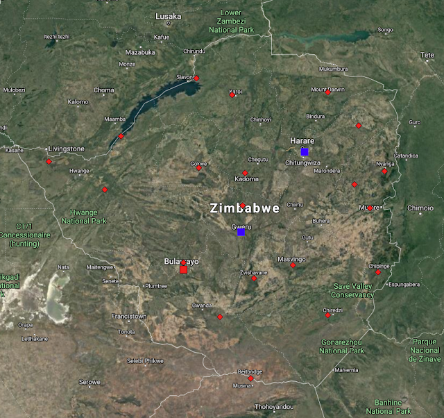
Fig. 79.1: The (approximate) locations of the weather stations in Zimbabwe. Those stations with a high warming trend between 1901 and 2000 are marked in red while those with a cooling or stable trend are marked in blue. Those denoted with squares are long stations with over 1200 months of data, while diamonds denote stations with over 360 months of data.


Overall there are only three long stations in Zimbabwe with over 1200 months of data, as well as a further sixteen medium stations with over 480 months of data, and another five with over 360 months of data (for a list of stations in Zimbabwe see here). The geographical locations of these 24 stations are indicated on the map in Fig. 79.1 above. As can be clearly seen, the stations are fairly evenly spread across the country. This means that a simple average of their temperature anomalies should yield a reasonably accurate value for the mean temperature anomaly (MTA) for the country as a whole.

The method used to determine the MTA was the same as that used in previous posts and outlined in Post 47. First, the monthly reference temperatures (MRTs) were calculated for each station time series using data from a suitable time interval; one that ensured that the maximum number of stations had a qualifying amount of good data within that time interval. In this case the thirty year period from 1971 to 2000 was selected as this ensured that all but two of the 24 station records could be used. The one station with the most significant data to be excluded was Salisbury (Berkeley ID: 44434). This station has an interesting dataset for reasons that I may explain in a later post.

As usual, a minimum of twelve years of data from within the specified thirty year time interval (1971-2000) was required to determine the MRTs for each station in order for data from that month and that station to be included in the MTA calculation. The MRTs for each set of station data were then subtracted from the raw monthly temperature readings to produce the anomaly time series for that station location. The anomaly time series from all the station records were then averaged to determine the MTA. This MTA data is shown in Fig. 79.2 below.


Fig. 79.2: The temperature trend for Zimbabwe relative to the 1971-2000 monthly averages based on an average of anomalies from stations with over 360 months of data. The best fit is applied to the monthly mean data from 1916 to 1975 and has a negative gradient of -0.96 ± 0.20 °C per century.


The MTA data in Fig. 79.2 appears to show a downward trend of about 1°C per century before 1980 followed by a temperature rise of about 1.5 °C. However, as Fig. 79.3 below indicates, the number of stations that contribute to the MTA drops significantly as you go back in time before 1960. This in turn suggests that the trend in Fig. 79.2 after 1960 is much more reliable than that before 1930.


Fig. 79.3: The number of station records included each month in the mean temperature anomaly (MTA) trend for Zimbabwe in Fig. 79.2.


As usual I have compared my results based on the raw temperature data from each station (see Fig. 79.2) with the Berkeley Earth (BE) version based on their adjusted data. The equivalent average of the BE adjusted anomalies is shown below in Fig. 79.4. From 1970 onwards its moving average (orange curve) is qualitatively very similar to the trend from the raw temperature data shown in Fig. 79.2 above (yellow curve), although the temperature rise seen in the raw data in Fig. 79.2 is about 50% greater. However, the trends before 1970 are markedly different. While the raw data in Fig. 79.2 exhibits a cooling of almost 0.6°C between 1920 and 1970, the BE data shows a slight warming.


Fig. 79.4: Temperature trends for Zimbabwe based on Berkeley Earth adjusted data. The average is for anomalies from all stations with over 360 months of data. The best fit linear trend line (in red) is for the period 1911-2010 and has a gradient of +0.85 ± 0.04°C/century.


The difference in the two temperature trends is illustrated below in Fig. 79.5. This shows how the adjustments made to the raw data by Berkeley Earth have added about 0.8°C of warming prior to 1980, and then removed a similar amount after 2000.


Fig. 79.5: The contribution of Berkeley Earth (BE) adjustments to the anomaly data in Fig. 78.4 after smoothing with a 12-month moving average. The blue curve represents the total BE adjustments including those from homogenization. The linear best fit (red line) to these adjustments for the period 1901-1980 has a positive gradient of +0.99 ± 0.02 °C per century. The orange curve shows the contribution just from breakpoint adjustments.


While the temperature trend based on BE adjusted data (Fig. 79.4) differs markedly from the one derived using raw data (Fig. 79.2), there is, however, excellent agreement between the data trends presented in Fig. 79.4 and the official BE version that is shown in Fig. 79.6 below. Both graphs are based on the same BE adjusted anomaly data, although the plot in Fig. 79.6 will likely have used a lot more data from station records with short time series (i.e. less than 360 months). However, because these time series are very short and noisy, they usually add very little new information to the temperature trend over time. That is why I (rightly) ignore them.

In addition, the averaging processes used to combine the adjusted anomalies into an MTA were probably very different. I constructed the anomaly time series shown in Fig. 79.4 by using a simple average of all the anomaly time series with over 360 months of data. In contrast, the BE version shown in Fig. 79.6 was probably constructed using techniques such as gridding, interpolation and homogenization. The data in Fig. 79.6 have also been converted to mean temperatures by adding on the mean annual temperature value for the country (which is about 21.3°C) to all the MTA data. Yet despite all these potentially significant differences, the two results are remarkably similar (other than the 21.3°C offset obviously).


Fig. 79.6: The temperature trend for Zimbabwe since 1840 according to Berkeley Earth.


This degree of similarity between the data in Fig. 79.4 and Fig. 79.6 therefore implies that the simple averaging process that I have used to construct the MTAs in both Fig. 79.2 and Fig. 79.4 is just as accurate as the more sophisticated procedures that Berkeley Earth use to construct mean temperature time series such as that presented in Fig. 79.6 above. But this is not a new result. I have shown that the same in true for BE adjusted data from most countries. The key criterion for the two averaging methods to agree is for the geographical spread of stations within the country or region to be sufficiently uniform so that all stations have equal area weightings. In the case of Zimbabwe this is clearly the case, as Fig. 79.1 above illustrates. This then validates the simple averaging process used for the raw data in Fig. 79.2 because it is the same process as was used for Fig. 79.4, and it uses data from the same stations with the same geographical distribution.


Summary

The data in Fig. 79.2 shows that there is clearly strong warming of almost 1.5°C in Zimbabwe after 1980, but before 1980 the climate appears to have cooled.

Overall this suggests that at least some of the warming seen in Zimbabwe after 1980 is probably real as it coincides with the period of greatest anthropogenic carbon dioxide production. It is also similar in timing to temperature rises seen in MTAs elsewhere around the world as I have shown previously on this blog, although its magnitude is somewhat larger than is normally seen elsewhere.

Likewise, the cooling before 1980 is similar to temperature trends seen in neighbouring countries and much of the Southern Hemisphere.

The other major question that arises is, how much of this temperature rise post-1980 is due to carbon dioxide induced climate change, and how much is just natural variation similar to the decline seen before 1980?


Acronyms

BE = Berkeley Earth.

MRT = monthly reference temperature (see Post 47).

MTA = mean temperature anomaly.

Thursday, September 30, 2021

78. Mozambique - temperature trend 0.6°C WARMING after 1980

According to climate science, Mozambique has experienced a more or less continuous warming to its climate of over 1.2°C over the last 130 years. The reality as evidenced by the actual temperature data is rather different. Like many places around the world, Mozambique has certainly seen some modest warming of about 0.6°C since 1980, but before 1980 the picture is uncertain, and on balance there may have been no significant warming at all in this period.

Mozambique has eleven long and medium weather stations most of which are located on, or near, the coast, as indicated in Fig. 78.1 below. This is same number of long and medium weather stations that was seen for Madagascar (see Post 77). However Madagascar also has another nine stations with over 300 months of data; Mozambique has only four.


Fig. 78.1: The (approximate) locations of the weather stations in Mozambique. Those stations with a high warming trend between 1901 and 2000 are marked in red while those with a cooling or stable trend are marked in blue. Those denoted with squares are stations with over 1000 months of data, while diamonds denote stations with over 480 months of data.


Of the eleven long and medium stations in Mozambique, two are long stations with over 1200 months of data, another two have over 1000 months of data, and the remaining seven are medium stations with over 480 months of data. Averaging the temperature anomalies from these eleven station records results in the mean temperature anomaly (MTA) for the region shown in Fig. 78.2 below. The method used to determine the MTA was the same as that used in previous posts and has been outlined in Post 47. 

First the monthly reference temperatures (MRTs) were calculated for a suitable time interval, in this case the thirty year period from 1951 to 1980. This ensured that all eleven long and medium temperature records contained sufficient valid data in this interval for each month (a minimum of twelve years of data for each MRT is usually required). The MRTs for each set of station data were then subtracted from the raw monthly temperature readings to produce the anomalies for that station location. The anomalies from all eleven long and medium station records were then averaged to determine the MTA.


Fig. 78.2: The temperature trend for Mozambique relative to the 1951-1980 monthly averages based on an average of anomalies from stations with over 480 months of data. The best fit is applied to the monthly mean data from 1913 to 2012 and has a positive gradient of +1.07 ± 0.06 °C per century.


The MTA data in Fig. 78.2 appears to show an upward trend of about 1°C per century, but that is not the whole story. As Fig. 78.3 below indicates, the number of stations that contribute to the MTA drops significantly as you go back in time before 1950. This in turn suggests that the trend in Fig. 78.2 after 1960 is much more reliable than that before 1930.


Fig. 78.3: The number of station records included each month in the mean temperature anomaly (MTA) trend for Mozambique in Fig. 78.2.


As usual I have compared my results based on raw temperature data with the Berkeley Earth (BE) version based on their adjusted data. The equivalent average of the BE adjusted anomalies is shown below in Fig. 78.4. From 1940 onwards it is very similar to the trend from the raw temperature data shown in Fig. 78.2 above. In both cases the MTA plateaus between 1940 and 1980 before rising by about 0.8°C over the next twenty years. Then it drops back slightly by about 0.2°C in the following decade.


Fig. 78.4: Temperature trends for Mozambique based on Berkeley Earth adjusted data. The average is for anomalies from all stations with over 360 months of data. The best fit linear trend line (in red) is for the period 1911-2010 and has a gradient of +1.00 ± 0.03°C/century.


The MTA based on BE adjusted data also shows good agreement between 1920 and 1990 with the official Berkeley Earth trend for Mozambique shown in Fig. 78.5 below. It is only after 1995 that there is significant disagreement between the two plots. This may be because Berkeley Earth has included more data in the average after 2000 using many more stations with less than 300 months of data than I have.


Fig. 78.5: The temperature trend for Mozambique since 1840 according to Berkeley Earth.


It is clear that the temperature trend for Mozambique exhibits some warming after 1980, but the trend before 1980 is less clear. However, if we look at all the available data (see here for a list of all stations in Mozambique) we do see that there are a number of stations with data from 1930 to 1960 that are not included in the MTA trend shown in Fig. 78.2 above, due to insufficient data within the MRT period. It turns out that the temperature time series of most of these station datasets display cooling trends from 1930-1960. The one main exception is the data from Lourenço Marques (Berkeley Earth ID: 156935) which shows more or less continuous warming from 1920 onwards.

If we wish to incorporate these extra stations into the MTA then we need to change the MRT period to the interval 1931-1960 when most of this extra data was recorded. This is what I have done to generate the data in Fig. 78.6 below. The other significant change was to discard the data from Lourenço Marques (aka Maputo) from the MTA. The reason for doing this was that, while this station clearly has the longest set of temperature data in Mozambique (it has temperature data from as far back as 1892), its temperature trend is an outlier. This is probably because the station is located in the capital city Maputo and is more prone to the urban heat island (UHI) effect than most other stations in the country. I should note that this outlier behaviour of capital cities is not unusual. The same was seen for Jakarta in Indonesia (see Post 31) as well as for Sydney and Melbourne in Australia.


Fig. 78.6: The mean temperature trend relative to the 1931-1960 monthly averages for stations in Mozambique with over 300 months of data but excluding Lourenço Marques. The best fit is applied to the monthly mean data from 1921 to 1980 and has a positive gradient of +0.16 ± 0.12 °C per century.


The result of this change of MRT, together with the removal of the data from Lourenço Marques, is to completely change the temperature trend before 1940 (see Fig. 78.6 above). While the trend after 1980 still exhibits a warming of 0.6°C, the trend before 1980 is now neutral but with significant natural variability. It is also more reliable as it is based on data from more stations than previously (see Fig. 78.7 below). This would suggest that the temperature trend in Fig. 78.7 is a better representation of the true behaviour of the Mozambique climate over the last 100 years than is the trend in Fig. 78.2. It also provides more evidence to suggest that anthropogenic climate change is really only a post-1980 phenomenon and not one that began in 1850.


Fig. 78.7: The number of station records included each month in the mean temperature anomaly (MTA) trend for Mozambique in Fig. 78.6.


Summary

The data shows that there is clearly strong warming of almost 0.6°C in Mozambique after 1980 (see Fig. 78.2).

Before 1980 the climate appears to be stable (see Fig. 78.6).

Overall this suggests that the warming seen in Mozambique after 1980 is probably real as it coincides with the period of greatest anthropogenic carbon dioxide production. It is also similar in timing and magnitude to temperature rises seen elsewhere around the world as I have shown previously.


Acronyms

BE = Berkeley Earth.

MRT = monthly reference temperature (see Post 47).

MTA = mean temperature anomaly.