146: Spain - temperature trends COOLING before 1980

The analysis of temperature data for Portugal in the previous post appeared to indicate that the local climate had warmed continuously since 1870 by over 1°C in total. The caveat to this was the poor data quantity before 1940 with only two stations of significance contributing data to the regional trend, and one of them, Lisbon, clearly displayed characteristics in its data that were suggestive of the urban heat island effect. 

In this post I will look at the corresponding temperature data for Portugal's neighbour, Spain, to see if the temperature trends seen in Post 145 are repeated, as would be expected of neighbouring territories. The results will in fact show that they are not, and that the trends for Portugal before 1940 are probably wrong. In fact the data for Spain indicates that the climate cooled over the one hundred years before 1980 and has only recently begun to warm.

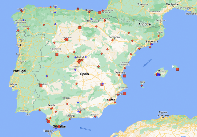
Spain has many more weather stations compared to Portugal, which given the difference in size is not surprising. Despite this, the station densities of the two countries are roughly the same. Spain has fourteen long stations with over 1200 months of data before 2014 and another 69 medium stations with over 480 months of data. The locations of these stations are indicated on the map in Fig. 146.1 below. They include two stations in Gibraltar and four in the Balearic Islands. They are distributed fairly evenly across the country but there are significant clusters around Madrid and south of Seville. 

Fig. 146.1: The (approximate) locations of the 83 longest weather station records in Spain. Those stations with a high warming trend between 1911 and 2010 are marked in red while those with a cooling or stable trend are marked in blue. Those denoted with squares are long stations with over 1200 months of data, while diamonds denote medium stations with more than 480 months of data.

In order to quantify the changes to the climate of Spain the temperature anomalies for all stations with over 480 months of data before 2014 were determined and averaged. This was done using the usual method as outlined in Post 47 and involved first calculating the temperature anomaly each month for each station relative to its monthly reference temperature (MRT), and then averaging those anomalies to determine the mean temperature anomaly (MTA) for the whole country for each month. The MRTs for each station in Spain were calculated using the same 30-year period, namely from 1961 to 1990. The resulting MTA is shown as a time series in Fig. 146.2 below and clearly shows that temperatures were decreasing for over 110 years up until 1980. After which they appear to increase suddenly by about 0.8°C.

Fig. 146.2: The mean temperature change for Spain since 1780 relative to the 1961-1990 monthly averages. The best fit is applied to the monthly mean data from 1871 to 1980 and has a slight negative gradient of -0.19 ± 0.10 °C per century.

The total number of stations included in the MTA in Fig. 146.2 each month is shown in Fig. 146.3 below. The peak in the frequency around 1970 suggests that the 1961-1990 interval was indeed the most appropriate to use for the MRTs. It also indicates that data from at least ten stations were used to calculate the MTA for almost every month back to 1865. As fifteen stations appears to the minimum number needed to provide an accurate MTA, this suggests that the trend in Fig. 146.2 is reliable at least as far back as 1865.

Fig. 146.3: The number of station records included each month in the mean temperature anomaly (MTA) trend for Spain in Fig. 146.2.

If we next consider the change in temperature based on Berkeley Earth (BE) adjusted data we get the MTA data in Fig. 146.4 below. This again was determined by averaging each month the anomalies from the 83 longest stations and suggests that the climate was warming before 1980. This clearly contradicts the raw data in Fig. 146.2.

Fig. 146.4: Temperature trends for Spain based on Berkeley Earth adjusted data. The best fit linear trend line (in red) is for the period 1871-1980 and has a positive gradient of +0.32 ± 0.04°C/century.

But if we next compare the curves in Fig. 146.4 with those from the published Berkeley Earth (BE) version for Spain shown in Fig. 146.5 below, we see that there is excellent agreement between the two sets of data at least as far back as 1865. This indicates that the simple averaging of adjusted anomalies used to generate the BE MTA in Fig. 146.4 is as effective and accurate as the more complex gridding method used by Berkeley Earth in Fig. 146.5. In which case simple averaging should be just as effective and accurate in generating the MTA using raw unadjusted data in Fig. 146.2.

Fig. 146.5: The temperature trend for Spain since 1750 according to Berkeley Earth.

The differences between the MTA in Fig. 146.2 and the BE versions using adjusted data in Fig. 146.4  are instead mainly due to the data processing procedures used by Berkeley Earth. These include homogenization, gridding, Kriging and most significantly breakpoint adjustments. These lead to changes to the original temperature data, the magnitude of these adjustments being the difference in the MTA values seen in Fig. 146.2 and Fig. 146.4. The magnitudes of these adjustments are shown graphically in Fig. 146.6 below. The blue curve is the difference in MTA values between adjusted (Fig. 146.4) and unadjusted data (Fig. 146.2), while the orange curve is the contribution to those adjustments arising solely from breakpoint adjustments. Both are considerable with the former leading to an additional warming since 1865 of over 0.5°C.

Fig. 146.6: The contribution of Berkeley Earth (BE) adjustments to the anomaly data in Fig. 146.4 after smoothing with a 12-month moving average. The blue curve represents the total BE adjustments including those from homogenization. The linear best fit (red line) to these adjustments for the period 1871-1980 has a positive gradient of +0.506 ± 0.013 °C per century. The orange curve shows the contribution just from breakpoint adjustments.

The overall impact of the BE adjustments can be seen more clearly if we compare the 5-year averages for the raw data (from Fig. 146.2) and the BE adjusted data (from Fig. 146.4). This comparison is shown in Fig. 146.7 below. It clearly shows that the trend based on adjusted data (red curve) exhibits considerably more warming since 1870.

Fig. 146.7: The 5-year mean temperature change for Spain since 1820 based on the original raw data from Fig. 146.2 (in blue) and the Berkeley Earth adjusted data from Fig. 146.4 (in red).

Summary

The raw unadjusted temperature data for Spain clearly shows that the climate cooled by about 0.2°C from 1870 to 1980 (see Fig. 146.2)

In contrast, the BE adjusted data claims that the climate warmed by 0.3°C over the same period (see Fig. 146.4).

After 1980 the climate has clearly warmed by about 0.8°C (see Fig. 146.7).

The results presented here clearly disagree with those for Portugal in Post 145. However, as the MTA for Portugal before 1960 is based on data from less than five stations compared to two or three times as many stations for Spain, that would suggest that the Spain data is the more accurate.

Acronyms

BE = Berkeley Earth.

MRT = monthly reference temperature (see Post 47).

MTA = mean temperature anomaly.

Long station = a station with over 1200 months (100 years) of data before 2014.

Medium station = a station with over 480 months (40 years) of data before 2014.

List of all stations in Spain with links to their raw data files.

133: UHI #6 - Buenos Aires (Argentina)

The second largest city in South America by population is Buenos Aires in Argentina with a population of over thirteen million people. The largest is Sao Paulo in Brazil. Both could be categorized as urban heat islands (UHIs); Sao Paulo in particular has warmed by about 3°C since 1887 and Buenos Aires by up to 2°C. However, as I have yet to fully analyse temperature data from Brazil it is not possible for me to compare the Sao Paulo data to the temperature change for the wider region, although this is unlikely to be more than about 1°C. So instead I will concentrate on Buenos Aires. Sao Paulo will come later.

A comparison of the temperature trends for Buenos Aires and Argentina shows that temperatures have risen far more in Buenos Aires than they have in Argentina as a whole. In fact as Fig. 133.1 below shows, they have risen almost three times faster in Buenos Aires since 1900 than they have in Argentina. Before 1900 temperatures were stable in both Buenos Aires and Argentina.

Fig. 132.1: The change to the 5-year average temperatures of Buenos Aires (red curve) and Argentina (blue curve) since 1900.

In Post 61 I examined the temperature trends for Argentina. The mean temperature change since 1900 is shown in Fig. 132.2 below and it indicates that Argentina has exhibited only modest warming over the last one hundred years. The best fit for 1901-2000 indicates a temperature rise of about 0.64°C while the 5-year average suggests a rise of about 0.52°C.

Fig. 132.2: The mean temperature change for Argentina since 1900 relative to the 1961-1990 monthly averages. The best fit is applied to the monthly mean data from 1901 to 2000 and has a positive gradient of +0.64 ± 0.11 °C per century.

The oldest major weather station in Argentina is Buenos Aires Observatorio (Berkeley Earth ID: 151642). It is located in the heart of Buenos Aires and has continuous data stretching back as far as 1856, although there is a break in the data between 2006 and 2011. It is one of only two major stations within 20 km of the city centre, hence its significance as a case study of the urban heat island (UHI) effect. The other is Aeroparque (Berkeley Earth ID: 151640) which only has data from 1961 onwards but also exhibits strong warming.

In contrast to the rest of Argentina, Buenos Aires Observatorio shows strong and continuous warming since 1910 (see Fig. 132.3 below). Before 1910 the temperatures were stable. The best fit for 1901-2000 indicates a temperature rise of about 2.4°C in one hundred years while the 5-year average suggests a rise of 1.77°C.

Fig. 132.3: The mean temperature change for Buenos Aires Observatorio since 1900 relative to its 1961-1990 monthly averages. The best fit is applied to the monthly mean data from 1901 to 2000 and has a positive gradient of +2.40 ± 0.18 °C per century.

Summary

The following temperature changes were observed from 1901 to 2000.

Argentina: 0.52°C (trend 0.64°C).

Buenos Aires: 1.77°C (trend 2.40°C).

So Buenos Aires has warmed by almost 1.8°C more than the surrounding state of Argentina, or more than three times faster. A classic UHI!

129: UHI #2 - Melbourne (Victoria)

The Australian state of Victoria has a total population of 6.7 million, of which 5.1 million live in the city of Melbourne. That means that 76% of the population of Victoria live in its capital city even though Melbourne accounts for only 4.4% of the area of Victoria. It is not really surprising then that the temperature trends for Melbourne and Victoria over the last 100 years are markedly different. In fact while the state of Victoria has cooled slightly for most of the last 120 years, Melbourne has warmed by over 2°C (see Fig. 129.1 below). So like Sydney in the previous post, Melbourne looks like a classic urban heat island (UHI).

Fig. 129.1: The change to the 5-year average temperatures of Melbourne (red curve) and Victoria (blue curve) since 1900.

 

In Post 19 I examined the temperature trends for Victoria. The mean temperature change since 1880 is shown in Fig. 129.2 below and it indicates that Victoria has exhibited no significant warming. In fact the best fit for 1886-2005 indicates that temperatures actually declined very slightly, although the 5-year average over the same period suggests that they may have risen slightly by about 0.47°C with most of this rise occurring after 1990.

Fig. 129.2: The mean temperature change for Victoria since 1880 relative to the 1966-1995 monthly averages. The best fit is applied to the monthly mean data from 1886 to 2005 and has a slight negative gradient of -0.02 ± 0.08 °C per century.

The mean temperature anomaly (MTA) for Victoria shown in Fig. 129.2 above is the result of averaging monthly temperature anomalies from over fifty stations as Fig. 129.3 below demonstrates (see here for a list of all stations). However, before 1900 there are less than twenty available stations so the MTA is less reliable and more prone to error from statistical variability. For more details and analysis of the complete data for Victoria see Post 19.

Fig. 129.3: The number of station records included each month in the mean temperature anomaly (MTA) trend for Victoria in Fig. 129.2.

The oldest weather stations in Victoria is Melbourne Regional Office (Berkeley Earth ID: 151813). It is located in the heart of Melbourne and has continuous data stretching back as far as 1855. It is also the only major station within 20 km of the city centre that has continuous data extending back before 1940 (the next best is Laverton Aerodrome), hence its significance as a case study of the urban heat island (UHI) effect.

In contrast to the rest of Victoria, Melbourne Regional Office shows significant and continuous warming since 1880 (see Fig. 129.4 below). The best fit for 1886-2005 indicates a temperature rise of more than 1.4°C in 120 years while the 5-year average suggests a rise of over 2.1°C.

Fig. 129.4: The mean temperature change for Melbourne Regional Office since 1880 relative to its 1966-1995 monthly averages. The best fit is applied to the monthly mean data from 1886 to 2005 and has a positive gradient of +1.23 ± 0.10 °C per century.

Summary

The following temperature changes were observed from 1886 to 2005.

Victoria: 0.47°C (trend -0.02°C).

Melbourne: 2.1°C (trend 1.48°C).

So Melbourne has warmed by at least 1.5°C more than the surrounding state of Victoria, or up to four times faster. A classic UHI!

Given that both Sydney and Melbourne appear to be great examples of UHIs, one might expect the same of similar large cities, Adelaide and Brisbane. Yet this appears not to be the case. Neither of these cities exhibits greater warming than the rest of their respective states even though over 70% of the South Australian population of 1.8 million live in Adelaide. For Brisbane and Queensland, though, the proportion is only 44%, although Brisbane is almost twice the size of Adelaide by population. The reason both Adelaide and Brisbane do not exhibit striking UHI properties could be that they are too small. Adelaide has a population that is less than a quarter of that of Sydney. That said, the population of Perth in Western Australia is just less than two million and yet as the next post will show, it too appears to be an urban heat island (UHI).

128: UHI #1 - Sydney (New South Wales)

In my previous post I explained the concept of the urban heat island (UHI). Unfortunately, finding clear examples in the global temperature records is not so easy. This is not because they don't exist, but because to demonstrate their existence beyond a reasonable doubt requires good data for both the urban area and the wider region within which the UHI sits. 

In the case of the urban data, this needs to be from a station that is located in the heart of the urban area and not on its perimeter such as at the local airport. Finding datasets from such locations is a lot harder than one might think because most weather stations are deliberately sited away from the centre of urban areas. Then the dataset needs to be sufficiently long with no gaps in the record in order for it to exhibit a definite trend over time. 

In the case of the regional data, this too needs to be based on long datasets with no gaps in their records. But in addition, a large number of these datasets are needed in order to establish an accurate trend for the region.

Satisfying these criteria is particularly difficult in the Southern Hemisphere where the data for most countries other than Australia is not particularly good. Nevertheless, I have identified six examples in the Southern Hemisphere so far (excluding Brazil which I have yet to examine in detail) where the quality of the temperature data for the UHI and its host country or state is sufficient to detect unambiguous differences in their temperature trends. Over the following six posts, including this one, I will examine each of these six examples in turn. So for Exhibit #1 I give you Sydney in New South Wales (NSW), Australia.

The city of Sydney has a population of about 5.3 million. That means that 65% of the New South Wales (NSW) population of 8.2 million live in Sydney even though Sydney accounts for only 1.5% of the area of NSW. It is not really surprising then that the temperature trends for Sydney and NSW over the last 100 years are markedly different. For while NSW has barely warmed at all in the last 140 years, Sydney has warmed by almost 2°C (see Fig. 128.1 below).

Fig. 128.1: The change to the 5-year average temperatures of Sydney (red curve) and New South Wales (blue curve) since 1900.

In Post 18 I examined the temperature trends for New South Wales. The mean temperature change since 1880 is shown in Fig. 128.2 below and it indicates that NSW has exhibited no significant warming. In fact the best fit for 1886-2005 indicates a temperature rise of less than 0.12°C in 120 years while the 5-year average suggests a rise of about 0.25°C.

Fig. 128.2: The mean temperature change for New South Wales since 1880 relative to the 1965-1994 monthly averages. The best fit is applied to the monthly mean data from 1886 to 2005 and has a slight positive gradient of +0.099 ± 0.077 °C per century.

The mean temperature anomaly (MTA) for NSW shown in Fig. 128.2 above is the result of averaging monthly temperature anomalies from over one hundred stations as Fig. 128.3 below demonstrates (see here for a list). However, before 1880 there are less than twenty available stations so the MTA is less reliable and more prone to error from statistical variability. For more details and analysis of the complete data for NSW see Post 18.

Fig. 128.3: The number of station records included each month in the mean temperature anomaly (MTA) trend for New South Wales in Fig. 128.2.

One of the oldest weather stations in NSW is Sydney Observatory Hill (Berkeley Earth ID: 151986). It is located in the heart of Sydney, south of the opera house and harbour, and has continuous data stretching back as far as 1859. It is also the only major station within 20 km of the city centre, hence its significance as a case study of the urban heat island (UHI) effect. 

In contrast to the rest of NSW, Sydney Observatory Hill shows significant and continuous warming since 1880 (see Fig. 128.4 below). The best fit for 1886-2005 indicates a temperature rise of more than 1.2°C in 120 years while the 5-year average suggests a rise of over 1.5°C.

Fig. 128.4: The mean temperature change for Sydney Observatory Hill since 1880 relative to its 1965-1994 monthly averages. The best fit is applied to the monthly mean data from 1886 to 2005 and has a positive gradient of +1.01 ± 0.08 °C per century.

Summary

The following temperature changes were observed from 1886 to 2005.

NSW: 0.25°C (trend 0.12°C).

Sydney: 1.5°C (trend 1.2°C).

So Sydney has warmed by at least 1°C more than NSW, or up to ten times faster. A classic UHI!

124: Arctic temperature trends - a comparison

In the previous five posts I examined the temperature changes for five different territories in the Arctic region (Greenland, Iceland, the Faroe Islands, Jan Mayen and Svalbard). All appeared to exhibit similar trends with a peak in temperatures in the 1930s followed by a dip, and then another rise after 1980. In this post I will compare and examine these five trends in more detail.

In Post 11 I demonstrated how the correlation between temperature trends from different stations depends on their separation: the further apart they are, the less well correlated they are. In fact if the distance between them exceeds 1500 km their correlation becomes very weak. On that basis we would not expect any great correlation between the the Faroes and Svalbard as they are over 2,000 km apart. In contrast, Greenland, the Faroes and Jan Mayen are all less than 600 km from Iceland, so the correlations of their temperature data with that from Iceland should be must stronger. The trends in Fig. 124.1 below attempts to do just that, compare the trends of Greenland, the Faroes and Jan Mayen with that of Iceland. For clarity the trends of Greenland and the Faroes are offset vertically by -3°C and +3°C respectively, as are their Icelandic comparator curves.

Fig. 124.1: The 5-year moving average temperature trends for Greenland, Jan Mayen and the Faroe Islands all compared against the equivalent trend for Iceland.

The data in Fig. 124.1 can be summarized as follows.

The trends of Greenland, Jan Mayen and the Faroe Islands all appear to follow the same broad pattern. Temperatures peak in the 1930s, then decline by about 2°C by the 1980s before peaking again after 2000. Only in Jan Mayen is the peak after 2000 higher (by about 0.5°C) than the one in the 1930s.

The trend from the Faroe Islands is most closely correlated with that of Iceland. Not only is the broad trend the same, but the smaller peaks and troughs also align well.

The smaller peaks for Greenland are not closely correlated with those of Iceland or the other two regions. This may be because the mean temperature anomaly (MTA) for Greenland is the result of averaging anomalies from stations over a much larger area than is the case for Iceland, Jan Mayen and the Faroe Islands. So some of the fine detail may be lost by the averaging of stations that are themselves not well correlated.

Jan Mayen shows better correlation with Iceland but its peaks and troughs are larger in size. This may be the result of it having a more extreme climate (due to being inside the Arctic Circle) where the temperature anomalies are naturally larger.

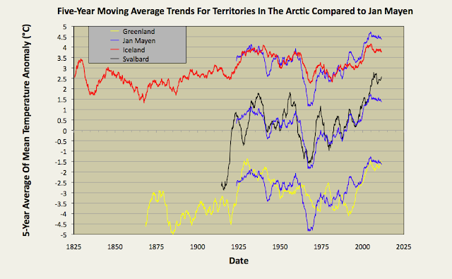
Fig. 124.2: The 5-year moving average temperature trends for Greenland, Iceland and Svalbard all compared against the equivalent trend for Jan Mayen.

If we repeat the process used for Fig. 124.1 but instead use the temperature trend of Jan Mayen as the reference comparator, then we get the trends shown in Fig. 124.2 above.

What we see from Fig. 124.2 is similar to what we saw in Fig. 124.1 with temperatures peaking in the 1930s, then declining by about 2°C by the 1980s before peaking again after 2000.

Once again the smaller peaks for the trend of Greenland are not closely correlated with those of the comparator (in this case Jan Mayen), and the reason is probably the same.

This time, though, the greatest correlation of the smaller peaks and troughs in each trend line is between those for Jan Mayen and Svalbard. This is perhaps not a surprise given that they are near(-ish) neighbours and both are well inside the Arctic Circle.

Summary and conclusions

The general long-term temperature trends of Greenland, Iceland, Jan Mayen and the Faroe Islands are well correlated over timescales of more than 20 years. This suggests that there is no need to adjust the temperature data because the data is correct.

Correlations on shorter timescales (5-10 years) are generally weaker. The two notable exceptions are firstly Jan Mayen and Svalbard, and secondly Iceland and the Faroe Islands.

123: Svalbard - temperature trends STABLE to 2000

One of the most notable features of Svalbard is its location. It is one of the most northerly inhabited regions on the planet, located 900 km from the North Pole and almost 1000 km from the northern coast of Norway. As a result it is probably the best source of temperature data that we have for the Arctic, particularly given that there is no significant temperature data available within a radius of 800 km of the North Pole as I showed in Post 118.

That said, there are only seven  stations in Svalbard that have over 480 months of data. Of these only two have over 1000 months of data with one being a long station with over 1200 months of data. The remaining five are medium stations with over 480 months of data (for a list see here). Although the Svalbard archipelago is a part of Norway, its distance from Norway implies that its climate is likely to be rather different. For that reason I am studying it separately in this post rather than with Norway (which I will examine later).

Fig. 123.1: The mean temperature change for Svalbard since 1900 relative to the 1956-1985 monthly averages. The best fit is applied to the monthly mean data from 1921 to 2000 and has a negative gradient of -0.46 ± 0.37 °C per century.

 

What the data that we do have for Svalbard tells us is that the change in climate since 1920 is very similar to that seen for Jan Mayen in Post 122. The climate cooled slightly until 2000 and then warmed by about 2°C (see Fig. 123.1 above). However this warming is still smaller in magnitude than the variations seen in the 5-year average of up to 4°C.

In order to quantify the changes to the climate of Svalbard the temperature anomalies for each of the seven stations with the most data were determined and averaged. This was done using the usual method as outlined in Post 47 and involved first calculating the temperature anomaly each month for each station, and then averaging those anomalies to determine the mean temperature anomaly (MTA) for the region. The anomalies were determining relative to the monthly reference temperatures (MRTs) using a set reference period, in this case from 1956 to 1985. The total number of stations included in the MTA in Fig. 123.1 each month is indicated in Fig. 123.2 below. The peak in the frequency between 1970 and 1980 suggests that the 1956-1985 interval was indeed the most appropriate to use for the MRTs.

 

Fig. 123.2: The number of station records included each month in the mean temperature anomaly (MTA) trend for Svalbard in Fig. 123.1.

 

The locations of the seven stations with the most temperature data are shown in the map in Fig. 123.3 below. Most stations are clustered around Barentsburg with two situated on the outer islands of Hopen to the southeast and Bear Island (as in the Alistair Maclean novel and film) to the south.

 

Fig. 123.3: The (approximate) locations of the seven longest weather station records in Svalbard. Those stations with a high warming trend between 1911 and 2010 are marked in red while those with a cooling or stable trend are marked in blue. Those denoted with squares are long stations with over 1200 months of data, while diamonds denote medium stations with more than 480 months of data.

 

If we next consider the change in temperature based on Berkeley Earth (BE) adjusted data we get the MTA data shown in Fig. 123.4 below. This again was determined by averaging each monthly adjusted anomaly from the seven longest stations in Svalbard. The mean temperature follows a similar trajectory to that of the unadjusted data in Fig. 123.1 with temperatures over a 10-year average (orange curve) fluctuating by over 2°C and a large peak occurring around 1930. Temperatures in 2010 are also about 0.5°C higher than in 1930.

 

Fig. 123.4: Temperature trends for Svalbard based on Berkeley Earth adjusted data. The best fit linear trend line (in red) is for the period 1921-2000 and has a negative gradient of -0.72 ± 0.15°C/century.

 

Comparing the curves in Fig. 123.4 with the published Berkeley Earth (BE) version for Svalbard and Jan Mayen in Fig. 123.5 below shows that there is good agreement between the two sets of data even though Fig. 123.5 includes data from Jan Mayen. This indicates that the simple averaging of anomalies used to generate the BE MTA in Fig. 123.4 is as effective and accurate as the more complex gridding method used by Berkeley Earth in Fig. 123.5. In which case simple averaging should be just as effective and accurate in generating the MTA using raw unadjusted data in Fig. 123.1 even though the geographical distribution of stations is far from homogeneous, as was shown in Fig. 123.3. What is truly remarkable about the graph in Fig. 123.5 below is that it suggests that Berkeley Earth thinks it can determine the mean temperatures for Svalbard and Jan Mayen as far back as 1760 even though there is no data before 1910.

 

Fig. 123.5: The temperature trend for Svalbard and Jan Mayen since 1750 according to Berkeley Earth.

 

The similarity in the two sets of data, Fig. 123.1 and Fig. 123.4, is reflected in the scale of the adjustments made to the original data by Berkeley Earth. The magnitudes of these adjustments are shown graphically in Fig. 123.6 below. The blue curve is the difference in MTA values between adjusted (Fig. 123.4) and unadjusted data (Fig. 123.1), while the orange curve is the contribution to those adjustments arising solely from breakpoint adjustments.

In this case neither set of adjustments is particularly large. The most significant adjustment is for data after 1990 which is adjusted downwards apparently to reduce the extent of the temperature rise seen after 1990 in Fig. 123.1. The other significant adjustment is for data between 1940 and 1960. The effect of this appears to be to reduce the size of the temperature peak before 1960. Neither of these adjustments significantly affect the overall trend of the data other than to reduce the warming after 2000 to values similar to those seen in BE adjusted trends for other regions.

 

Fig. 123.6: The contribution of Berkeley Earth (BE) adjustments to the anomaly data in Fig. 123.4 after smoothing with a 12-month moving average. The blue curve represents the total BE adjustments including those from homogenization. The linear best fit (red line) to these adjustments for the period 1921-2000 has a slight negative gradient of -0.13 ± 0.03 °C per century. The orange curve shows the contribution just from breakpoint adjustments.

 

Summary

According to the raw unadjusted temperature data, the climate of Svalbard has remained fairly stable since 1930 with possibly some cooling, but may have warmed by up to 2°C since 2000 (see Fig. 123.1). Any warming since 2000 is still comparable to the natural variations in temperature seen over the previous eighty years.

Over the same period the adjusted temperature data from Berkeley Earth appears to show similar climatic variations (see Fig. 123.4) to the unadjusted (see Fig. 123.1).

Berkeley Earth has estimated the climate variations for Svalbard as far back as 1760 (see Fig. 123.5) despite there being no reliable temperature data before 1910.

The patterns seen in the temperature data for Svalbard in Fig. 123.1 (decline before 1990 and warming after) are similar to those seen previously for nearby islands of Greenland (Fig. 119.1 in Post 119), Iceland (Fig. 120.1 in Post 120), the Faroes (Fig. 121.1 in Post 121) and Jan Mayen (Fig. 122.2 in Post 122).



Acronyms

BE = Berkeley Earth.

MRT = monthly reference temperature (see Post 47).

MTA = mean temperature anomaly.

Link to list of all stations in Svalbard and their raw data files.

122: Jan Mayen - temperature trends VARIABLE

The Norwegian island of Jan Mayen lies in the Arctic Circle approximately 600 km northeast of Iceland, 500 km east of Greenland and almost 1000 km from the coast of Norway. It is just over 50 km long and is inhabited only by a few Norwegian military and meteorological personnel on six month deployments. It does, though, have two weather stations (BE ID: 16234 and BE ID: 157312 with 735 and 1113 months of data respectively) that provide the only temperature data for over 500 km in all directions (see Fig. 122.1 below).

 

Fig. 122.1: The (approximate) locations of the two longest weather station records in Jan Mayen. Those stations with a high warming trend between 1911 and 2010 are marked in red while those with a cooling or stable trend are marked in blue.

 

The mean temperature anomaly (MTA) for Jan Mayen is shown in Fig. 122.1 below. From 1920 to 1990 the temperature trend is downward with temperatures falling by about 0.7°C according to the best fit line (red line) or 1.5°C according to the 5-year moving average (yellow line). After 1990 the temperature increases by up to 2°C. Both of these changes are less than the natural variation seen in the 5-year average (yellow curve) so it is impossible to definitively attribute them to climate change.

 

Fig. 122.2: The mean temperature change for Jan Mayen since 1920 relative to the 1971-2000 monthly averages. The best fit is applied to the monthly mean data from 1921 to 2000 and has a negative gradient of -0.93 ± 0.25 °C per century.

The MTA in Fig. 122.2 is the average of anomaly data from two stations (see Fig. 122.3 below) and was determined using the usual method as outlined in Post 47. The anomalies were determined relative to monthly reference temperatures (MRT) with the MRTs calculated using data from 1971-2000.

Fig. 122.3: The number of station records included each month in the mean temperature anomaly (MTA) trend for Jan Mayen in Fig. 122.2.

 

Repeating the averaging process using data that has been adjusted by Berkeley Earth (BE) yields the temperature curve shown in Fig. 122.4 below. In this case the 10-year average (orange curve) is broadly similar in shape to the yellow curve in Fig. 122.2, but the temperature fall before 1990 and the rise after are both slightly larger. In both cases, however, the temperatures in 2010 are less than 0.5°C higher than in 1930.

 

Fig. 122.4: Temperature trends for Jan Mayen based on Berkeley Earth adjusted data. The best fit linear trend line (in red) is for the period 1921-2000 and has a negative gradient of -1.04 ± 0.11°C/century.

 

The similarity in the two sets of data (Fig. 122.2 and Fig. 122.4) is reflected in the scale of the adjustments made to the original data by Berkeley Earth. The magnitudes of these adjustments are shown graphically in Fig. 122.5 below. The blue curve is the difference in MTA values between adjusted (Fig. 122.4) and unadjusted data (Fig. 122.2), while the orange curve is the contribution to those adjustments arising solely from breakpoint adjustments. In this case neither are particularly large, with data after 1950 being adjusted down by about 0.18°C. The only significant adjustment is for data between 1960 and 1976 which is adjusted upwards by about 0.9°C. The effect of this is to reduce the size of the temperature dip before 1970 seen in Fig. 122.2.

 

Fig. 122.5: The contribution of Berkeley Earth (BE) adjustments to the anomaly data in Fig. 122.4 after smoothing with a 12-month moving average. The blue curve represents the total BE adjustments including those from homogenization. The linear best fit (red line) to these adjustments for the period 1921-2000 has a slight negative gradient of -0.07 ± 0.04 °C per century. The orange curve shows the contribution just from breakpoint adjustments.

 

Summary

According to the raw unadjusted temperature data, the climate of Jan Mayen has remained fairly stable since 1930 (see Fig. 122.2).

Over the same period adjusted temperature data from Berkeley Earth appears to show similar climate variations (see Fig. 122.5).

The patterns seen in the temperature data for Jan Mayen in Fig. 122.2 (decline before 1990 and warming after) are similar to those seen previously for nearby islands of Greenland (Fig. 119.1 in Post 119), Iceland (Fig. 120.1 in Post 120) and the Faroes (Fig. 121.1 in Post 121).



Acronyms

BE = Berkeley Earth.

MRT = monthly reference temperature (see Post 47).

MTA = mean temperature anomaly.

121: Faroe Islands - temperature trends STABLE

The longest temperature record in the Faroe Islands is from a station at Thorshavn. It has nearly 1800 months of data, but no other temperature record in the islands has more than 435 months of data. In fact only another two (at Vagar and Akraberg) have more than 120 months of data (see here for a list). This means that the temperature record for the Faroe Islands is heavily dependent on the Thorshavn data with the other two stations only affecting the mean temperatures after 1980. 

The result is the time series for the mean temperature anomaly (MTA) shown in Fig. 121.1 below. What is striking is that the general form of the five-year moving average (yellow curve) is very similar to those for both Greenland (see Fig. 119.1 in Post 119) and Iceland (see Post 120.1 in Post 120). Temperatures declined from 1930 until 1990 and then rebounded. In all three cases the temperatures today are no higher than in the 1930s but the amount of cooling from 1930-1990 is different, being highest for Greenland and least for the Faroe Islands. This is not a surprise, though, as it is well known that climates that are more extreme (i.e. Greenland) experience larger temperature fluctuations than are seen in more temperate climes (i.e. the Faroe Islands).

Fig. 121.1: The mean temperature change for the Faroe Islands since 1920 relative to the 1981-2010 monthly averages. The best fit is applied to the monthly mean data from 1931 to 2010 and has a negative gradient of -0.40 ± 0.15 °C per century.

In order to quantify the changes to the climate of the Faroe Islands the temperature anomalies for the three longest station records were averaged. This was done using the usual method as outlined in Post 47 and involved first calculating the temperature anomaly each month for each station, and then averaging those anomalies to determine the mean temperature anomaly (MTA) for the region.

The process of determining the MTA in Fig. 121.1 involved first determining the monthly reference temperatures (MRTs) for each station using a set reference period, in this case from 1981 to 2010, and then subtracting the MRTs from the raw temperature data to deliver the anomalies. The total number of stations included in the MTA in Fig. 121.1 each month is indicated in Fig. 121.2 below. The peak in the frequency after 1980 illustrates why the 1981-2010 interval was indeed the most appropriate to use for the MRTs.

Fig. 121.2: The number of station records included each month in the mean temperature anomaly (MTA) trend for the Faroe Islands in Fig. 121.1.

If all the data is considered, the MTA trend for the Faroe Islands will have data extending back to 1867 as shown in Fig. 121.3 below. Much of the data before 1930 indicates that temperatures then, at least for Thorshavn, were cooler than in the 1930s and to day. Again this is similar to the results from Greenland and Iceland, but it is unclear how much of this temperature change is genuine warming of the climate and how much is just the result of natural fluctuations. But the fact that these features are repeated in multiple regions means that they cannot be discounted as being isolated results that are the result of poor measurements.

Fig. 121.3: The mean temperature change for the Faroe Islands since 1860 relative to the 1981-2010 monthly averages. The best fit is applied to the monthly mean data from 1871 to 2010 and has a positive gradient of +0.27 ± 0.07 °C per century.

The locations of the three stations used to determine the MTA in Fig. 121.3 are shown in the map in Fig. 11214 below. The temperature data from all three appear to exhibit modest warming trends, but this is mainly due to the fitting intervals used in each case. Vagar and Akraberg only have data after 1970 where the MTA in Fig. 121.3 is warming. The trend for Thorshavn was for data from 1911-2010, and is therefore biased by the fact that the fitting interval does not extend from peak to peak. This is akin to fitting to a sine wave as I explained with Fig. 4.7 in Post 4. So the positive trend is not real.

Fig. 121.4: The (approximate) locations of the three longest weather station records in the Faroe Islands. Those stations with a high warming trend between 1911 and 2010 are marked in red while those with a cooling or stable trend are marked in blue. Those denoted with squares are long stations with over 1200 months of data, while diamonds denote stations with more than 240 months of data.

If we next consider the change in temperature based on Berkeley Earth (BE) adjusted data we get the MTA data shown in Fig. 121.5 below. This again was determined by averaging each monthly anomaly from the three longest stations in the Faroe Islands. The mean temperature follows a similar trajectory to that of the unadjusted data in Fig. 121.3 with temperatures fluctuating by over 1°C and a large peak occurring around 1930. However the BE adjustments appear to have lowered this peak relative to temperatures in 2010 by over 0.25°C compared to the raw data in Fig. 121.3.

Fig. 121.5: Temperature trends for the Faroe Islands based on Berkeley Earth adjusted data. The best fit linear trend line (in red) is for the period 1871-2010 and has a positive gradient of +0.61 ± 0.03°C/century.

Comparing the curves in Fig. 121.5 with the published Berkeley Earth (BE) version for the Faroe Islands in Fig. 121.6 below shows that there is good agreement between the two sets of data. However, Berkeley Earth appear to think they can determine the temperature back to 1760 even though there is no data before 1860. Who says climate scientists are pessimists?

Fig. 121.6: The temperature trend for the Faroe Islands since 1750 according to Berkeley Earth.

The differences between the MTA in Fig. 121.3 and the BE versions using adjusted data in Fig. 121.5  can be determined by calculating the difference in the MTA values seen in Fig. 121.3 and Fig. 121.5. The result is shown graphically in Fig. 121.7 below. The blue curve is the difference in MTA values between adjusted (Fig. 121.5) and unadjusted data (Fig. 121.3), while the orange curve is the contribution to those adjustments arising solely from breakpoint adjustments. What is clear is that there is only one significant adjustment. That is a breakpoint adjustment of over 0.25°C made to the Thorshavn data in 1951. The difference between the blue and orange curves in Fig. 121.7 is due to the difference in MRT interval used in Fig. 121.3 and by Berkeley Earth in Fig. 121.5.

Fig. 121.7: The contribution of Berkeley Earth (BE) adjustments to the anomaly data in Fig. 121.5 after smoothing with a 12-month moving average. The blue curve represents the total BE adjustments including those from homogenization. The linear best fit (red line) to these adjustments for the period 1871-2010 has a positive gradient of +0.330 ± 0.005 °C per century. The orange curve shows the contribution just from breakpoint adjustments.

Summary

According to the raw unadjusted temperature data, the climate of the Faroe Islands has cooled from 1930 to 1980 by about 1°C. It then warmed by a similar but slightly smaller amount until 2005 (see Fig. 121.1).

Over the same period adjusted temperature data from Berkeley Earth appears to show that the climate of the Faroe Islands has warmed by over 0.25°C since 1930 and over 1°C since the 1800s (see Fig. 121.5).

The difference in the raw unadjusted data (Fig. 121.3) and the adjusted data (Fig. 121.5) is mainly due to a single breakpoint adjustment of 0.26°C in 1951.

Any warming trend since 1870 is small (~0.3°C) compared to what look like natural temperature variations (~1°C). The origin of these variations (shown in Fig. 121.3) is uncertain but cannot be the result of greenhouse gas emissions when those emissions were so low compared to today. However, similar patterns are seen in the temperature data of nearby islands of Greenland (Post 119), Iceland (Post 120). and Jan Mayen (from 1920 only), so these features seen in the data before 1930 may be real and representative of synchronous climate variations occurring across the North Atlantic/Arctic region.



Acronyms

BE = Berkeley Earth.

MRT = monthly reference temperature (see Post 47).

MTA = mean temperature anomaly.

Link to list of all stations in the Faroe Islands and their raw data files.

120: Iceland - temperature trends COOLING before 2000

It is tempting to think of Iceland as being Greenland's little brother. This is not just because Iceland is smaller and close to Greenland, but also because their changes in climate over the last two hundred years are very similar. Like in Greenland, the climate of Iceland cooled from 1930 to 1990 before the mean temperatures rebounded. And like in Greenland, the mean temperatures today are no higher than they were in the 1930s (see Fig. 120.1 below).

Fig. 120.1: The mean temperature change for Iceland since 1920 relative to the 1971-2000 monthly averages. The best fit is applied to the monthly mean data from 1931 to 2000 and has a negative gradient of -1.43 ± 0.24 °C per century.

In order to quantify the changes to the climate of Iceland the temperature anomalies for each of the 21 stations with the most data (over 300 months) were determined and averaged. This was done using the usual method as outlined in Post 47 and involved first calculating the temperature anomaly each month for each station, and then averaging those anomalies to determine the mean temperature anomaly (MTA) for the region. The MTA since 1920 is shown as a time series in Fig. 120.1 above and clearly shows that temperatures declined continuously from 1930 to 1990 before levelling off and then rebounding.

The process of determining the MTA in Fig. 120.1 involved first determining the monthly reference temperatures (MRTs) for each station using a set reference period, in this case from 1971 to 2000, and then subtracting the MRTs from the raw temperature data to deliver the anomalies. If a station had at least twelve valid temperatures per month within the MRT interval (1971-2000) then its anomalies were included in the calculation of the mean temperature anomaly (MTA). The total number of stations included in the MTA in Fig. 120.1 each month is indicated in Fig. 120.2 below. The peak in the frequency after 1980 suggests that the 1971-2000 interval was indeed the most appropriate to use for the MRTs, although 1981-2010 would have been equally appropriate.

Fig. 120.2: The number of station records included each month in the mean temperature anomaly (MTA) trend for Iceland in Fig. 120.1.

The data in Fig. 120.2 above indicates that after 1940 there were up to 21 active stations, but before 1940 there were less than about six with only one station being operational before 1870. As six is generally too low a number to produce a reliable trend, the MTA data in Fig. 120.1 was truncated with only data post-1920 being shown. However, if all the data is considered, the MTA trend will have data extending back to 1823 as shown in Fig. 120.3 below. Note also that the low number of stations before 1900 results in a much higher variance of points in Fig. 120.3 about the mean (yellow line). This is more evidence of the greater unreliability of this earlier data, which is why the plot shown in Fig. 120.1 is more statistically reliable.

Fig. 120.3: The mean temperature change for Iceland since 1820 relative to the 1971-2000 monthly averages. The best fit is applied to the monthly mean data from 1841 to 2000 and has a positive gradient of +0.71 ± 0.08 °C per century.

The locations of the 21 stations used to determine the MTA in Fig. 120.3 are shown in the map in Fig. 120.4 below. Of these 21 stations, six are long stations with over 1200 months of data before 2014, and a further five are medium stations with over 480 months of data. The stations are evenly distributed across the island with most on, or near, the coast.

Fig. 120.4: The (approximate) locations of the 21 longest weather station records in Iceland. Those stations with a high warming trend between 1911 and 2010 are marked in red while those with a cooling or stable trend are marked in blue. Those denoted with squares are long stations with over 1200 months of data, while diamonds denote stations with more than 300 months of data.

If we next consider the change in temperature based on Berkeley Earth (BE) adjusted data we get the MTA data shown in Fig. 120.5 below. This again was determined by averaging each monthly anomaly from the 21 longest stations in Iceland. The mean temperature follows a similar trajectory to that of the unadjusted data in Fig. 120.3 with temperatures fluctuating by over 1°C and a large peak occurring around 1930. However the BE adjustments appear to have lowered this peak slightly relative to temperatures in 2010 when compared to the raw data in Fig. 120.3.

Fig. 120.5: Temperature trends for Iceland based on Berkeley Earth adjusted data. The best fit linear trend line (in red) is for the period 1841-2010 and has a positive gradient of +0.51 ± 0.03°C/century.

 

Comparing the curves in Fig. 120.5 with the published Berkeley Earth (BE) version for Iceland in Fig. 120.6 below shows that there is good agreement between the two sets of data. This indicates that the simple averaging of anomalies used to generate the BE MTA in Fig. 120.5 is as effective and accurate as the more complex gridding method used by Berkeley Earth in Fig. 120.6. In which case simple averaging should be just as effective and accurate in generating the MTA using raw unadjusted data in Fig. 120.1.

Fig. 120.6: The temperature trend for Iceland since 1750 according to Berkeley Earth.

Most of the differences between the MTA in Fig. 120.3 and the BE versions using adjusted data in Fig. 120.6  are mainly due to the data processing procedures used by Berkeley Earth. These include homogenization, gridding, Kriging and most significantly breakpoint adjustments. These lead to changes to the original temperature data, the magnitude of these adjustments being the difference in the MTA values seen in Fig. 120.3 and Fig. 120.5.

The magnitudes of these adjustments are shown graphically in Fig. 120.7 below. The blue curve is the difference in MTA values between adjusted (Fig. 120.5) and unadjusted data (Fig. 120.1), while the orange curve is the contribution to those adjustments arising solely from breakpoint adjustments. Both result in a consistent upward trend after 1920 with the former leading to an additional warming since 1930 of up to 0.25°C. These adjustments are, however, much smaller in total than the natural variation seen in the raw data in Fig. 120.3, so while they change the overall magnitude of the climate changes slightly, the general form of the temperature trends in Fig. 120.5 and Fig. 120.3 look broadly similar.

Fig. 120.7: The contribution of Berkeley Earth (BE) adjustments to the anomaly data in Fig. 120.5 after smoothing with a 12-month moving average. The blue curve represents the total BE adjustments including those from homogenization. The linear best fit (red line) to these adjustments for the period 1921-2010 has a positive gradient of +0.234 ± 0.007 °C per century. The orange curve shows the contribution just from breakpoint adjustments.

Summary

According to the raw unadjusted temperature data, the climate of Iceland has cooled from 1930 to 1990 by about 1°C. It then warmed by a similar but slightly smaller amount until 2005 (see Fig. 120.1).

Over the same period adjusted temperature data from Berkeley Earth appears to show that the climate of Iceland has warmed only fractionally since 1930, but by up to 2°C since the 1800s (see Fig. 120.5).

The reliability of the temperature data before 1930 is debatable due to the low number of stations and the large jumps in temperature that occur repeatedly. The origin of these jumps is uncertain but cannot solely be the result of greenhouse gas emissions when those emissions increased the atmospheric carbon dioxide concentration by so little compared to today.


Acronyms

BE = Berkeley Earth.

MRT = monthly reference temperature (see Post 47).

MTA = mean temperature anomaly.

Link to list of all stations in Iceland and their raw data files.