91. The Schwarzschild equation and scattering

In Post 86 I showed how the Greenhouse Effect can be viewed as resulting from a combined process of absorption of infra-red radiation by molecules of carbon dioxide (CO₂), followed by re-emission of the same wavelength of radiation, but in a different random direction. The law that leads to this result is the principle of detailed balance. I also showed how this process resembled a scattering process, but with a much greater strength due to the significantly greater absorption cross-section (σ_a) of CO₂ compared to its cross-section for Rayleigh scattering, σ_s. Therefore it could be modelled as a scattering process, but one with an appropriately large cross-section.

Then in Post 88 I showed how this combined process of absorption and re-emission resulted in absorption that decreased linearly with distance x into a gas of uniform density, rather than exponentially as predicted by the Beer-Lambert law. The importance of this result is that it demonstrates that the transmission of radiation through an absorbing gas will be greater than that predicted by the Beer-Lambert law, and so changes to the concentration of the absorbing gas will have a larger impact on the overall transmission than the Beer-Lambert law would predict. 

Sadly this result has been questioned by some who have claimed that the scattering (or combined absorption and re-emission) approach is not valid as it does not follow from, or agree with, Schwarzschild's equation. This equation is possibly named after the German physicist Karl Schwarzschild (shown below), although it could actually be named after his son Martin Schwarzschild who worked in the field of stellar evolution. In this post I will show that this claim of non-validity is not true and that Schwarzschild's equation leads to the exact same results as I outlined in Post 88.

 Fig. 91.1: Karl Schwarzschild (1873-1916)

The Model

In order to understand the Greenhouse Effect we need to consider the radiation flows through a thin layer of gas of thickness δx at some altitude x, and then extend this to model to the gas as a whole. In particular, we need to consider radiation flows through the gas from opposing directions. This is because each thin layer of the gas only absorbs a small fraction of radiation passing through it. Most of the rest is then absorbed by subsequent layers above the initial layer. However, after absorption the radiation is re-emitted and the re-emission process occurs equally in both directions (up and down). This means that some of this emitted radiation will travel in a downwards direction and reheat the first layer from the opposite direction. This is why the Beer-Lambert law fails.

In order to model this process we need to consider radiation fluxes in both directions as shown in Fig. 91.2 below. Let's assume that the gas has a concentration or particle density n(x), and each molecule of it has an absorption cross-section σ_a. If radiation of intensity I_u(x) travels in an upward direction from a hot surface and enters the gas layer from below, as shown in Fig. 91.2 below, a proportion of it will be absorbed by the gas. This in turn will heat the gas and cause it to emit radiation in both an upwards and a downwards direction. The result will be that the intensity of upward radiation leaving the gas layer will change by an amount δI_u(x).

Fig. 91.2: A schematic illustration of how scattering, absorption and thermal emission within each thin layer of the atmosphere alters the intensities of the upwelling (I_u) and downwelling (I_d) radiation.

The upwelling radiation will then go on to interact with gas above the layer shown in Fig. 91.2 and thus heat this gas as well. This gas will then re-emit radiation, some of it in a downward direction, and this downwelling radiation I_d(x) will then also pass through our original layer of gas. It in turn will be partially absorbed, heating the gas and causing it to radiate. The net result is that the intensity of the downwelling radiation leaving the gas layer will also change, in this case by an amount δI_d(x). So far this model is identical to the one outlined in Post 88. The next step is to consider the changes of intensity, δI_u(x) and δI_d(x), using Schwarzschild's equation and the Planck function, B(λ,T), where λ is the wavelength of the radiation and T is the temperature of the gas in kelvins at this height x. In the following discussion I will consider the absorption and re-emission of radiation at a fixed wavelength λ.

The Proof

As the upwelling radiation I_u(x) at a fixed wavelength λ passes through the thin layer of gas of thickness δx a small amount of it will be absorbed by the gas. This amount will be proportional to the number of molecules encountered per unit area, n(x)δx, their absorption cross-section, σ_a, and the amount of radiation in the original flux, I_u(x). The result is that the transmitted intensity will decrease by an amount equal to I_u(x)σ_an(x)δx.

At the same time the thin layer of gas will be emitting radiation in both the upward and downward direction due to its temperature T. This temperature will in turn vary with height x, so both B(λ,T) and I_u(x) will vary with x. The intensity emitted in each direction is given by the Planck function, B(λ,T), multiplied by the number of molecules per unit area in the layer, n(x)δx, and the emission cross-section, σ_e. The result of this emission process is that the transmitted intensity above the layer will increase by an amount equal to B(λ,T)σ_en(x)δx.

Combining these two effects of emission and absorption gives the total change in intensity of the upwelling radiation

δI_u(x) = [B(λ,T)σ_e - I_u(x)σ_a]n(x)δx

(91.1)

This is Schwarzschild's equation. However, it is only half the solution because there is a similar equation that can be derived for the changes to the downwelling radiation I_d(x) in the thin layer at the same wavelength λ. Thus the resulting equation will be

δI_d(x) = [B(λ,T)σ_e - I_d(x)σ_a]n(x)δx

(91.2)

Finally, there is one other consideration we must take into account: energy conservation at wavelength λ. The total energy flowing into the layer of gas must match the energy flowing out. This means that 

δI_u(x) + δI_d(x) = 0

(91.3)

and so

[ I_u(x) + I_d(x) ]σ_a = 2B(λ,T)σ_e 

(91.4)

We can now eliminate B(λ,T)σ_e from Eq. 91.1 and Eq. 91.2 and turn both equations into first order differential equtions. However, because the change in downwelling radiation I_d(x) in Fig. 91.2 is defined to be positive for changes of x in a negative direction the δx term must be negative, and therefore the differential term dI_d/dx = - δI_d/δx.This means that

 (91.5)

It then turns out that Eq. 91.5 is identical to Eq. 88.5 in Post 88. So if the equations are the same and the boundary conditions are the same, then the solutions must be the same as in Post 88. So even using Schwarzschild's equation as our starting point we end up with the same result. 

Finally, we can write Schwarzschild's equation as two differential equations, one for I_u(x) and one for I_d(x). From Eq. 91.1 we get the obvious result

(91.6)

The equivalent equation for I_d(x) is similar, but requires some explanation.

(91.7)

In Eq. 91.7 the order of the I(x)σ_a and B(λ,T)σ_e terms to the right of the equality sign have been reversed compared to Eq. 91.6. This is because the downwelling radiation, I_d(x), is flowing in the negative direction through the thin gas layer. So for I_u(x) the radiation term B(λ,T)σ_e is directed in the same direction as I_u(x) so it must be positive, while the absorption in the gas layer must leads to a lower value of I_u(x) above the layer than below. In the case of I_d(x) the reverse it true in both cases, hence the reversal of sign for both terms.

Finally, it should be noted that conditions of thermal equilibrium generally require the cross-sections σ_a and σ_e to be equal. This is particularly true for black body radiation where a black body at constant temperature must emit what it absorbs, otherwise it will gain or lose energy, and thus not be at constant temperature.

 

Implications

If we now apply the above results to a real system and consider the case of a column of gas of thickness L, and uniform density n that is independent of x, the model outlined above means that the upwelling radiation will vary with x through the gas as (see Post 88)

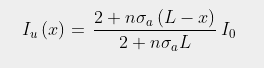
(91.8)

where I_o is the intensity of radiation entering the gas at x = 0, while the downwelling radiation will vary as

(91.9)

The difference between I_u(x) and I_d(x) will be constant (ΛI_o), as required by energy conservation, and will be equal to the amount transmitted at the end of the column (i.e. at x = L), so 

(91.10)

In Fig. 91.3 below I have suggested what I_u(x) and I_d(x) might look like through a 500 metre long horizontal column of air with 420 ppm of CO₂ when it is irradiated with 15 µm infra-red radiation from one end. It should be noted, though, that this theoretical data is based on an estimated value for the scattering cross-section of the CO₂ molecules that could be almost a factor of ten too small. Nevertheless, it still illustrates qualitatively how the transmission of 15µm infra-red radiation changes through the gas, and also how the Greenhouse Effect (as defined by the relative intensity of the reflected radiation at x = 0) is related to this transmission (see the red curve in Fig. 91.3).

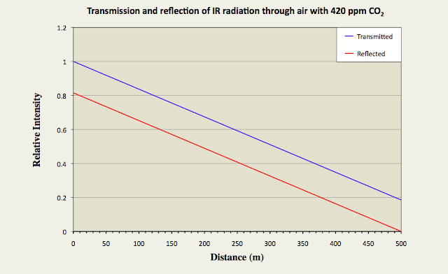
Fig. 91.3: The relative intensities of transmitted (I_u) and reflected (I_d) radiation along a 500 metre column of air containing 420 ppm of CO₂ with an absorption cross-section of 1.6 x 10^-24 m².

The graph in Fig. 91.3 suggests that a 500 metre column of air will transmit less than 18% of the incident radiation and reflect back the rest. The question is: is this more or less than that predicted by the Beer-Lambert law? The answer to this can be seen in Fig. 91.4 below.

Fig. 91.4: The relative intensities of radiation transmitted  through a column of air of length L containing 420 ppm of CO₂ with an absorption cross-section of 1.6 x 10^-24 m² based on two different models: (i) a backscattering model described by Eq. 91.10 (blue curve), and (ii) the Beer-Lambert law (red curve).

The blue curve in Fig. 91.4 demonstrates how the transmission through a column of air would decrease with the length of the column, L, if half of the absorbed radiation is backscattered or re-emitted in the reverse direction and half is re-emitted in the forward direction. The result is a curve that decays with L in accordance with Eq. 91.10. The red curve on the other hand shows how the transmission would change if it followed the (commonly accepted) Beer-Lambert law where the transmitted intensity varies with L as

(91.11)

What is clear is that the Beer-Lambert law underestimates the transmission for large values of L, and in effect predicts that there is no significant transmission beyond 400 metres. The blue curve shows that this is not the case with over 10% transmission for a column of length 1000 metres. In practice this means that the Beer-Lambert law will massively underestimate the impact of future increases in CO₂ levels because it will assume that the backscattering is already operating at close to 100% or saturation with 420 ppm of CO₂. Yet clearly it is not. In fact even at 10 km (the effective thickness of Earth's atmosphere) there is still more than 1% transmission. While this is small, it is not insignificant, particularly when considering the relatively small changes to the overall size of the Greenhouse Effect that are needed to create a warming of 1.5°C.

Caveats

The only condition I have applied to the proof and discussion described here is that set out in Eq. 91.4, which basically demands that each layer of the gas radiates the same amount of energy at each wavelength as it absorbs from the two fluxes, I_u(x) and I_d(x). This will be true provided all the heat of wavelength λ entering the gas originates from the Earth's surface at the bottom of Fig. 91.2, or at the very top of the atmosphere. In which case, the exact functional forms of I_u(x) and I_d(x) will depend only on the functional form of n(x) and the boundary conditions. However, at the top of the atmosphere this condition will not be satisfied as some of the incoming ultraviolet radiation from the Sun is absorbed there before it reaches the ground and so gets converted to infra-red radiation within the upper atmosphere. This means that Eq. 91.4 is no longer satisfied for each and every infra-red wavelength of interest within the gas.

In my next blog post I will consider a number of distinct and important examples to demonstrate how dependent the transmission is on the density profile of the gas, n(x), and also on the location of the heat source(s). These examples will also show that even when it sometimes looks like there is no Greenhouse Effect in operation, it is still there.

88. A scattering model of The Greenhouse Effect

In my two previous posts I analysed the structure of the 15 µm absorption band for carbon dioxide (CO₂) in order to demonstrate how increasing the concentration of CO₂ in the atmosphere increases the the band's width. This widening of the absorption band then slightly increases the proportion of infra-red radiation that is reflected back to the Earth's surface and thus increases the strength of the Greenhouse Effect, thereby increasing the surface temperature. As a result I showed that this enhancement is unlikely to contribute more than about 0.5°C to the strength of global warming, and probably contributes less than 0.2°C; i.e. much less than the 1.2°C that is claimed.

In this post I will consider a different impact of an increase to the atmospheric concentration of CO₂ by calculating the strength of the backscattering at the centre of the 15 µm absorption band. This will involve describing the mathematical and statistical basis for the Greenhouse Effect, and how it arises from the backscattering of photons by greenhouse gas molecules. As a result I will show just how little infra-red radiation within the 15 µm band can escape through the atmosphere, and so also show just how insensitive the backscattering and transmission of infra-red radiation are to further increases in the CO₂ concentration. Finally, I will calculate the expected temperature change for an increase in atmospheric CO₂ concentrations from 280 ppm to 420 ppm, and show that it is significantly less than 0.1°C.

How the scattering process works

The origin of the Greenhouse Effect is the interaction of infra-red photons with air molecules, specifically those of carbon dioxide (CO₂) and water vapour (H₂O). While all air molecules, including those of both oxygen and nitrogen, are capable of scattering infra-red photons via the process of Rayleigh scattering, this scattering is so weak at infra-red wavelengths that it is unimportant. In fact in Post 86 I showed that Rayleigh scattering at wavelengths of 15 µm is a million times weaker than that seen for visible light and which gives the daytime sky its blue colour.

Instead, the dominant process is one of absorption and re-emission of photons where air molecules absorb radiation, and then re-emit it in a random direction. This is only important at wavelengths that match both the peak in the thermal emission spectrum of the Earth's surface (from about 5 µm to 100 µm) and the excitation energies of the molecules. As only CO₂ and H₂O of the main components of the atmosphere have excitation energies that match the peak region of the thermal emission spectrum of the Earth's surface, they are the most important greenhouse gases.

As I showed in Post 86, the combined absorption and re-emission process results in radiation received from one direction (i.e. the Earth's surface) being redistributed in all directions with equal probability. This is because the time delay between absorption and re-emission means that the orientation of the emitting molecules could be in any random direction. The result is a process that looks just like random scattering, and because the direction of scattering is random it is determined by statistical probability.

One way to visualize the backscattering process is by considering the photons of outgoing infra-red radiation as particles that, every so often, collide with greenhouse gas molecules, and bounce off them at random angles. We can define the average distance photons travel between these collisions as the mean free path. At each collision half the phonons will be reflected back in the opposite direction from which they came, while the other half will be scattered forward. But eventually those that are scattered forward will collide with another molecule and half of those will also be backscattered. This process continues as the remaining forward scattered photons travel further into the medium or gas with more and more being reflected. The result is that, eventually almost all the photons have been reflected back, and virtually none are travelling in the original forward direction. This is how the backscattering process works.

It is important to acknowledge, however, that the real process that is occurring is not a backscattering one. The infra-red photons are actually being absorbed by CO₂ molecules which then become excited. They may then transfer this energy to other air molecules via collisions, but eventually those other air molecules will transfer the energy back to the CO₂ and the CO₂ molecules will re-emit it in some random direction. The time this process takes could be quite long, or very short, but it is happening so often that it will appear almost instantaneous. And therefore it will look just like scattering. 

The mathematics of scattering

In order to gauge the importance of this process we need to quantify it. That means defining the process mathematically. By doing so we will be able to see which factors affect the amount of backscattering, and in particular, how it depends on the thickness of the atmosphere and its CO₂ concentration.

In order to do this we must first construct a model of the atmosphere and consider a thin horizontal layer of the atmosphere of thickness δx at some arbitrary altitude x as shown in Fig. 88.1 below. In this model the density of carbon dioxide molecules is n(x), the intensity of the upwelling (or outgoing) radiation at a height x is I_u(x), and the intensity of the downwelling (or backscattered) radiation at the same height is I_d(x). 

Fig. 88.1: A schematic illustration of how scattering within each thin layer of the atmosphere alters the upwelling (I_u) and downwelling (I_d) intensities.

 

In thermal equilibrium the atmosphere will emit the same number of photons each second that it absorbs. This is the origin of the scattering process. Conservation of energy then dictates that the difference between I_u(x) and I_d(x) must be the same at all heights, x, and equal to the total intensity transmitted at the top of the atmosphere. It therefore follows that 

I_u(x) - I_d(x) = I_oΛ

(88.1)

where Λ is the effective total transmission coefficient of the atmosphere and I_o = I_u(0) is the total intensity of radiation emitted at the surface.

Now we consider the change in intensities of I_u(x) and I_d(x) as the radiation passes through the thin layer of thickness δx at height x (see Fig. 88.1 above). In each case there is a probability δp that each photon will be scattered where

δp =  n(x)σ_sδx

(88.2)

and σ_s is the scattering (or absorption) cross-section of the CO₂ molecule at the particular wavelength of the radiation being considered. For each photon that is scattered, half will be scattered forwards and half will be scattered backwards. This means that the value of I_u(x) will decrease by ½I_u(x)δp but increase by ½I_d(x)δp due to the backscattering of the reflected photons in I_d(x). For I_d(x) the opposite will be true. It therefore follows that the change in I_u(x) for a positive increase in x of δx will be

δI_u(x) = ½[I_d(x) - I_u(x)]n(x)σ_sδx

(88.3)

while the change in I_d(x) for a positive increase in x of δx will be (note the extra negative sign)

δI_d(x) = -½[I_u(x) - I_d(x)]n(x)σ_sδx

(88.4)

These results can be written in differential form as

 

(88.5)

The solution to Eq. 88.5 will depend on the distribution of the CO₂ molecules within the atmosphere, n(x), and the boundary conditions. The first boundary condition is I_u(0) = I_o and sets the amount of radiation that initially enters the atmosphere from the surface. The second is I_d(h) = 0 where h is the height of the atmosphere, and this states that once the radiation leaves the top of the atmosphere there can be no more backscattering. The final piece of information we need is the dependence of the CO₂ concentration on altitude, n(x).

The simplest model is to assume n(x) is constant (and equal to n_o) and thus independent of x. This is a fairly good approximation for the lower part of the troposphere and it is one I shall use as a starting point for the analysis. 

 

Transmission coefficient for a gas of uniform density

From Eq. 88.1 we can see that I_u(x) - I_d(x) must be a constant. As n(x) is a constant, Eq. 88.5 dictates that the first differentials of both I_u(x) and I_d(x) must be constant as well. It therefore follows that

(88.6)

The solution for I_d(x) must then be of the form I_d(x) = a(h - x) to satisfy both Eq. 88.6 and the boundary condition I_d(h) = 0, while Eq. 88.5 demands that a = ½ΛI_on_oσ_s. So

I_d(x) = ½ΛI_on_oσ_s(h - x)

(88.7)

The only unknown term is Λ, but we can determine it from Eq. 88.1 and the boundary condition for I_u(0) = I_o. 

From Eq. 88.1 we see that I_u(x) = a(h - x) + I_oΛ, which means that at x = 0 the condition I_o = ah + I_oΛ  must hold. This means that the fraction of radiation that is transmitted at the top of the atmosphere, Λ, is given by

(88.8)

If n_oσ_sh >> 2, then Λ ≈ 2/n_oσ_sh.

It also means that I_u(x) will have a negative linear dependence on x when x < h as follows

 (88.9)

while for x > h we find that the transmitted intensity is I_u(x) = I_oΛ. This negative linear dependence is very different from the exponential decay that is usually associated with pure absorption or attenuation of radiation and described by the Beer-Lambert law.

Knowing Λ allows us to estimate the percentage of infra-red radiation within the 15 µm absorption band that escapes through the atmosphere for different CO₂ concentrations, n_o. A CO₂ concentration of 280 ppm (as existed before 1750) equates to a CO₂ molecular concentration of n_o = 0.0118 mol/m³. The effective thickness of the atmosphere (h) at uniform density is approximately 10 km, while the scattering cross-section (σ_s) was estimated at around 1.6 x 10^-24 m² in Post 87. This gives a value for Λ of 1.67%. But if we instead consider a CO₂ concentration of 420 ppm (as exists today), n_o = 0.0177 mol/m³ and Λ = 1.12%. So an increase in the CO₂ concentration from 280 ppm to 420 ppm leads to the proportion of radiation being reflected by the 15µm CO₂ absorption band increasing from 98.33% to 98.88%. This will lead to a (small) increase in the surface temperature which we can now estimate.

In Post 86 I showed that the width of the 15 µm band typically extends from about 13.35 µm to 17.35 µm and thus reflects about 18.1% of all the infra-red radiation emitted by the Earth's surface. But that assumes that the reflectivity of the band is 100%. In fact it is only 98.88%, having risen from 98.33% due to the increase in atmospheric CO₂. This means that the increase in CO₂ will, in effect, have caused the feedback factor, f, to rise from 18.0% to its current value of 18.1%. We can then use this information, together with the Stefan-Boltzmann law, to determine the change in the surface temperature as we know that 1-f is inversely proportional to T⁴. What we find is that the temperature rise associated with this increase in reflectivity (and hence increase in f) is less than 0.09°C. In fact the actual rise will be probably be less than half this value due to the masking effect of the water vapour.

Result: Increasing the CO₂ concentration from 280 ppm to 420 ppm results in a global temperature increase of less than 0.09°C.

 

Transmission coefficient for a real atmosphere

The analysis so far has assumed that the atmosphere has a finite thickness of constant density that is independent of altitude. This, though, is not true for Earth. The increasing gravitational potential energy with increasing altitude means that fewer molecules have sufficient energy to reach high altitudes. The result is that the density of air decreases with height, and that dependence on height is exponential.

As carbon dioxide molecules are about 50% heavier than those of oxygen and nitrogen one might expect even fewer CO₂ molecules to be present by percentage at high altitudes, but this is not the case. The mixing ratio does not appear to change significantly with altitude. So if there are 420 molecules of CO₂ in every one million molecules of air at sea level, the same is true at heights of 10 km, 25 km, and 50 km. It is just that there are fewer numbers of all molecules at those altitudes.

Over the bottom 80 km of the atmosphere the molecular density, n(x), varies with altitude (x) as

n(x) = n_o e^-kx

(88.10)

where k = 1.4 x 10^-4 m^-1. The same dependence is seen for CO₂ with n_o = 0.0177 mol/m³ for an atmosphere containing 420 ppm of CO₂, and n_o = 0.0118 mol/m³ for an atmosphere containing 280 ppm of CO₂. The dependence of molecular density on altitude changes some of the mathematics outlined in the previous section, but both Eq. 88.1 and Eq. 88.5 will remain unaffected. The first change is to substitute Eq. 88.10 into Eq. 88.5 to give

(88.11)

It therefore follows that I_u(x) is given by

(88.12)

where c is a constant of integration. In which case I_d(x) will be

(88.13)

The values of c and Λ will be dictated by the boundary conditions, I_u(0) = I_o and I_d(h) = 0, which are the same as before. Consequently, the results for c and Λ are

(88.14)

and

(88.15)

It can be seen that if kh << 1, then Eq. 88.15 reduces to the same approximate form as Eq. 88.8, and so both the reflectivity and the temperature rise will be the same as before (see previous section). The more realistic scenario, though, is for kh >> 1, particularly if h > 80 km (in which case kh = 11.2). Then Eq. 88.15 reduces to

(88.16)

which if n_oσ_s >> 2k, then becomes Λ ≈ 2k/n_oσ_s. We can now calculate the expected temperature rise by following a similar procedure to that outlined at the end of the previous section. 

If n_o = 0.0118 mol/m³ (equivalent to a CO₂ concentration of 280 ppm), then Λ = 0.0232 and so 97.68% of the radiation at 15 µm is being absorbed and then reflected. However, if n_o = 0.0177 mol/m³ (equivalent to a CO₂ concentration of 420 ppm), then Λ = 0.0156. This means that an increase in the CO₂ concentration from 280 ppm to 420 ppm leads to the proportion of radiation being reflected by the 15µm CO₂ absorption band increasing from 97.68% to 98.44%. Given that the feedback factor for the 15 µm band is currently f = 0.181, this suggests that the previous value was 0.1796.

As the current mean temperature is 289 K, and the temperature must have increased by a factor of [ (1 - 0.1796)/(1 - 0.181) ]^1/4 due to the change in feedback factor, then the corresponding temperature rise must be only 0.12°C. Once again the masking effect of absorption by water vapour in the same frequency range as CO₂ will probably halve the real value of f from CO₂ . So a large increase in the CO₂ concentration will probably have less than half the effect on the mean global temperature than is stated here.

Result: Increasing the CO₂ concentration from 280 ppm to 420 ppm results in a global temperature increase of less than 0.12°C.

Conclusions

1) Increasing the atmospheric CO₂ concentration from 280 ppm to 420 ppm results in the infra-red transmission through the 15 µm absorption band reducing from 2.32% to 1.56%.

2) This leads to the 15 µm band reflecting back an extra 0.76% of the radiation within the borders of the band. But as the band only interacts with 10% of the outgoing infra-red radiation, this amounts to a total net increase of only 0.076% of all radiation being reflected.

3) This increase in reflection is only sufficient to raise global temperatures by 0.06°C.

NOTE: The above analysis assumes a scattering cross-section of σ_s = 1.6 x 10^-24 m². This unfortunately is just an estimate, and the true value could be up to an order of magnitude greater. Given the importance of this value to the whole theory of climate change one might think its value would be easily found and widely known, but unfortunately it is not. If σ_s is indeed greater by a factor of ten, then both Λ and the temperature increase due to the CO₂ concentration rising from 280 ppm to 420 ppm will be a factor of ten smaller.

86. How photons interact with carbon dioxide molecules

In my previous post (Post 85) I countered a number of myths surrounding the greenhouse effect, and outlined how it really works. Many people falsely believe that it is caused by a heating of the atmosphere by outgoing infra-red radiation, but this is not the case. The key concept at the heart of the greenhouse effect is photon scattering, or more accurately, the absorption and re-emission of infra-red photons by molecules of the greenhouse gases. There are three main gases that perform this role: carbon dioxide (CO₂), water vapour (H₂O), and methane (CH₄). Each of these compounds absorbs electromagnetic radiation at its own set of unique wavelengths, but it is the absorption in the wavelength range between 6 µm and 90 µm that is key as this is where 96% of the thermal emission from the Earth's surface takes place. As CO₂ is seen as the most important player in terms of anthropogenic greenhouse gas emissions I will consider its role in greatest detail.

The emission and absorption spectra

In Fig. 85.1 of Post 85 I showed the main absorption bands of carbon dioxide in the infra-red part of the electromagnetic spectrum. In total there are four main bands at 2 µm, 2.7 µm, 4 µm and 15 µm, but only the 15 µm band is of any importance as the other three have energies that are way beyond the peak of the infra-red emission spectrum for Earth's outgoing radiation. This is illustrated in Fig. 86.1 below, where the blue curve represents the Earth's emission spectrum at 289 K and the red curve shows which frequencies are absorbed by CO₂. The area under the blue curve thus represents the total power of the radiation emitted at the Earth's surface, while the area under the red curve is the amount of radiated heat that can be absorbed and then reflected by CO₂.

 

Fig. 86.1: The electromagnetic emission spectrum for the Earth's surface at a mean temperature of 289K (blue curve) together with the absorption profile due to CO₂ between 14.2 µm and 16.2 µm (red curve).

The graph in Fig. 86.1 shows that only the 15 µm band is important as it is the only one close to the radiation peak. It is centred at 667 wavenumbers. Note: wavenumbers are the number of wavelengths of a radiation type that can fit in a distance of one centimetre. They are used because they are a measure of frequency, they result in much smaller numbers compared to other units of frequency like hertz, and are proportional to the photon energy of the radiation. The absorption bands at 2 µm, 2.7 µm and 4 µm correspond to wavenumbers of 5000, 3704 and 2500 cm^-1 respectively. Consequently, they can only interact with the tail of the frequency spectrum where there is very little energy being emitted (i.e. less than 1% of the total).

What the curves in Fig. 86.1 show is that only about 9% of the Earth's outgoing radiation can be absorbed and then reflected back by the carbon dioxide molecules in the atmosphere. In other words, the area under the red curve is only 9% of the area under the blue curve. Yet in Post 85 I showed that in reality 59% of the radiation is reflected back. The difference in these two numbers is largely due to water vapour which not only accounts for most of that difference (i.e. 50%), but also overlaps the 15 µm absorption peak of CO₂ (see Fig. 85.1 in Post 85), and so may render much of its function redundant. This is one reason why the claim that increasing the amount of CO₂ in the atmosphere will necessarily increase the strength of the greenhouse effect is disputed by many.

 

Fig. 86.2: The absorption bands of carbon dioxide and water vapour at sea level.

 

The other complicating factor is the actual width of the 15 µm band. The peak of maximum absorption generally stretches from about 14.2 µm to 16.2 µm, or from about 700 to 620 wavenumbers (or a width of 10.8 meV), and results in a feedback factor f = 9.2% and a temperature rise of 6.88°C. 

The band width, though, is dependent on both temperature and pressure. The full band at its tails can stretch from 12.5 µm to 18.5 µm (800 to 540 wavenumbers or a width of 32.2 meV), but absorption in the outer parts of the band decreases dramatically (see Fig. 86.2 above). If we were to use the full width of the band to determine the backscatter it would result in 26.8% of the outgoing radiation being reflected (see Fig. 86.3 below) and a temperature rise of 21.7°C; still much less than the 59% backscatter and the 58°C temperature rise that is actually seen.

Fig. 86.3: The electromagnetic emission spectrum for the Earth's surface at a mean temperature of 289K (blue curve) together with the potential absorption profile due to CO₂ between 12.5 µm and 18.5 µm (red curve).

A more realist estimate would be achieved by considering the width at the half maximum points of the band. This will be from about 13.35 µm to 17.35 µm (749 to 576 wavenumbers or a width of 21.4 meV) and would result in an absorption and reflection of 18.1%. This equates to a temperature rise at the surface of the Earth of 14.1°C.

Backscattering by Rayleigh scattering

The photons of infra-red radiation emitted by the Earth's surface interact with the carbon dioxide in two ways. One is by elastic scattering and the other via absorption and re-emission.

In elastic scattering the photons basically bounce off the CO₂ molecules like the collision of two billiard balls. This is the basis of what is known as Rayleigh scattering, named after the nineteenth-century British physicist Lord Rayleigh (John William Strutt), and it is a result of the electromagnetic interaction of the photon with the charged particles (electrons and protons) in the molecule. After collision the photons will end up travelling in a different direction. Some will be reflected back while others will carry on in a forward direction. It is the ones that are reflected that contribute to the greenhouse effect. The intensity of photons at a distance R from the molecule after being scattered through an angle θ is given by the equation

(86.1)

It can be seen that the overall scattering probability depends on the wavelength of the radiation (λ) and the strength of the polarizability of the molecule doing the scattering (α). The strong inverse dependence on wavelength explains why the sky is blue in daylight. This happens because blue light photons with wavelengths of about 400 nm scatter sixteen times more often as they travel through the Earth's atmosphere than red light photons of wavelength 800 nm do. It also means that Rayleigh scattering from carbon dioxide at wavelengths of 15 µm is about a billion times less likely to occur than the scattering of visible light. This is because the wavelengths of the photons being scattered are at least twenty times greater, so the scattering rate of 15 µm photons by CO₂ molecules is at least 160,000 times less than for visible light. But in addition, the proportion of CO₂ in the atmosphere is only 0.042% of all the molecules. This equates to about 150 moles of CO₂ per square metre of the Earth's surface.

Another way of describing the strength of the scattering is via a scattering cross-section, σ_s. This is a measure of the effective cross-sectional area of each molecule that a photon will see, or alternatively how effective that molecule is at blocking the radiation. The scattering cross-section is usually (but not always) much less than the physical dimension of the molecule. 

Using the definition of scattering cross-section Eq. 86.1 becomes

(86.2) 

 

where the scattering cross-section, σ_s(λ,α) is a function of both the wavelength of the radiation (λ) and the polarizabilty (α) as follows

(86.3)

All molecules have their own unique polarizabilities; a list of some of the more common ones can be found here. Most of the common atmospheric gases have similar values for α, although the value for CO₂ is about 50% higher than most. So scattering from CO₂ is about twice that from oxygen and nitrogen. Nevertheless, this still means that with only about one in a billion 15µm photons being scattered by the 150 moles per square metre of CO₂, the Rayleigh scattering cross-section of CO₂ at this wavelength equates to only about 10^-35 m². This is a million billion times smaller than the actual size of the molecule.

The key point, therefore, is that Rayleigh scattering is of negligible importance when discussing the greenhouse effect because it is a billion times weaker than the Rayleigh scattering we see of visible light. Absorption and re-emission of photons by the 15 µm band are the more important processes, but as I will explain next, their combined behaviour in terms of scattering is very similar to Rayleigh scattering, but much stronger.

Backscattering by absorption and re-emission

Almost all backscattering by carbon dioxide occurs via a process of absorption and re-emission of the infra-red photons with wavelengths in the region of the 15 µm band (i.e. 12.5-18.5 µm). The closer these photons are in wavelength to the centre of the band the more strongly they are absorbed.

Once excited, the molecule may then collide with other molecules and exchange its extra energy with them, thereby heating the gas as a whole. But once all the gas is heated equally, thermal equilibrium will be established where some of the excited CO₂ molecules will re-emit photons at the same rate that other CO₂ molecules are absorbing them. This situation physicists refer to as the steady state. At this point, for every photon being absorbed, another is being re-emitted by another molecule in a random direction.

Ultimately, every molecule wants to get to its lowest energy state, so while bombarding it with radiation will force its energy state to increase, it also increases the rate at which it tries to lose energy. So eventually an equilibrium is achieved where the amount of radiation being absorbed by the gas balances the amount that is lost through re-emission. The key point to note, though, is that the re-emission is a random process that can result in the emitted photons being ejected in any direction. In contrast, most of the absorbed photons come from a single direction: the Earth's surface. This means that fewer of the re-emitted photons end up travelling away from the surface as some are reflected back. Those photons that are reflected back then provide additional heat to the surface, thereby raising its temperature even further. This is the origin of the Greenhouse Effect. 

 

Structure of the absorption band

The infra-red photons emitted from the Earth's surface are absorbed by carbon dioxide via a process of molecular excitation where the molecule is promoted to a higher energy state. Usually this process is in the form of electrons within the molecule moving to higher energy levels, but those transitions are usually of very high energy (several electron volts or eV) and so they only result from the absorption of visible or ultraviolet light. 

The 15 µm transition in carbon dioxide is in the infra-red part of the spectrum and so it is of a much lower energy (about 83 meV). Instead it results from a bond stretching excitation where the molecule bends, as shown in mode v₂ in Fig. 86.4 below, under the action of the incoming electromagnetic wave of the photon. This bond stretching occurs because of an uneven distribution of electric charge within the molecule which then interacts with the electric field of the incoming electromagnetic wave or photon.

Fig. 86.4: The three vibrational modes of carbon dioxide. The symmetric stretch mode (v₁) occurs at 7.5 µm but does not absorb because of symmetry violation. The bend mode (v₂) corresponds to absorption at 15 µm, while the asymmetric stretch mode (v₃) corresponds to absorption at 4.3 µm.

In addition to the bond stretching, a much smaller amount of energy from the incoming photon may go towards increasing the angular momentum or rotational spin of the molecule. This leads to "wings" or branches to the central band as shown in Fig. 86.5 below, with the lower energy branch being denoted as the P branch, and the higher energy one the R branch. It is these branches that cause the band to broaden from a single sharp peak Q at 15 µm to a broader band stretching from 12.5 µm to 18.5 µm.

 

Fig. 86.5: The detailed structure of the 15 µm absorption band for CO₂ showing the absorption peaks associated with rotational transitions.

 

The branches P and R are each comprised of a set of evenly spaced discrete transitions, each one matched to a different change in rotational energy of the molecule due to a change in its angular momentum state J by an amount ∆J = ±1. This is because the incoming photon has an angular momentum quantum of J = +1 and angular momentum must be conserved in the absorption process. The R branch arises from absorption processes where the photon causes the molecule to spin faster, while the P branch arises from absorption processes where the photon causes the molecule to spin more slowly (i.e. the angular momentum of the photon is in the opposite direction to that of the molecule). The two branches are, in theory, mirror images of each other, but in practice centrifugal distortion and rotational-vibrational coupling lead to the line spacing increasing at lower energies.

As the energy of each rotational state J of the molecule is (ideally) equal to J(J+1)hB where h is Planck's constant and B is given by

(86.4)

with I being the moment of inertia of the molecule about its spin axis, the energy change associated with a transition from state J to J+1 when a photon is absorbed will be ±2hB(J+1) (see here). So the absorption peaks due to changes in rotation have an ideal energy separation of 2hB, or about 1.54 wavenumbers (cm^-1) or 0.2 meV for lines in the 15 µm band of carbon dioxide. 

These individual line transitions are also broadened via doppler broadening due to the different speeds and directions of motion of the various molecules, and pressure broadening due to collisions with other molecules in the atmosphere. Both of these broadening mechanisms are temperature dependent and increase as the temperature increases. The result is that the width and overall scattering cross-section of each line will increase with temperature thereby narrowing or closing completely the gaps between the individual rotational lines in the spectrum. For lines in the 15 µm absorption band of CO2 the typical scattering cross-section is about 10^-23 m², which is about one trillion (i.e. 10¹²) times greater than the scattering cross-section of each molecule due to Rayleigh scattering at the same wavelength.

In addition, an increase in temperature will shift the position of the peak or maximum in both the P and R branches, J_max (again see here). This is because the height of each line in the 15 µm band is dependent on both its J number and the temperature. Each line has a degeneracy of 2J+1, while the probability of exciting that rotational J mode depends exponentially on both energy and temperature. This means that the relative occupancy of each mode, N_J, is given by 

(86.5)

where the energy E_J of the mode J is given by J(J+1)hB, N_o is the total number of excited modes, and Z is a normalization term that is equal to the sum of the probabilities.

 (86.6)

This also explains why the P and R branches in Fig. 86.5 have peaks in their distributions. The occupancy of each rotational state N_J increases linearly with J via the degeneracy term 2J+1, but for large J decreases more rapidly due to the energy term E_J in the exponential. This leads to a maximum in the distribution, the position of which relative to the band centre at Q can be determined by differentiation with respect to J. The result is given by 

(86.7)

What this shows is that as the temperature of the gas increases, the position of the maxima will move further from the band centre at Q, so the overall width of the band will increase with temperature as well. This is because higher temperatures will lead to a higher proportion of CO₂ molecules in higher energy rotational states with larger J values. Generally, though, it takes a large temperature change to significantly widen the band. As the position of the R branch maximum relative to Q increases with temperature T as √T, it is reasonable to expect the width of the band to do the same.

Finally, if the width of the absorption band can change with temperature, then it can also change with CO₂ concentration. In this case the width will be set by the highest value of J for which N_J exceeds some threshold value N_th, this being the number of modes required to almost completely absorb the outgoing radiation at that wavelength. According to Eq. 86.5 this will be the value of J such that

(86.8)

Rearranging Eq. 86.8 gives the following result for the threshold J value, J_th, that defines the edge of the band

(86.9)

So Eq. 86.9 not only confirms that the band width varies approximately as √T, but also that it varies approximately as √ln(N_o). 

Conclusions

The dominant mechanism by which CO₂ molecules scatter infra-red radiation in the 15 µm band is by absorption and re-emission.

The absorption and re-emission process has a similar effect to that of Rayleigh scattering, but it is almost a trillion (i.e. 10¹²) times stronger. 

The width of the 15 µm band increases with temperature as √T, but increases much more slowly with CO₂ concentration (see Eq. 86.9).