92. The Greenhouse Effect for real atmospheres

In my previous post I showed how Schwarzschild's equation for the absorption and emission of radiation by a gas could result in identical results to a model based purely on elastic scattering. The only conditions on the proof I presented were that the gas is only heated at one end, and that energy conservation applies within the gas; namely that the energy each layer of the gas emits by Planck radiation balances the total energy it absorbs from the two fluxes of upwelling and downwelling radiation, I_u(x) and I_d(x) respectively. I then showed that this leads to a higher transmission through thick layers of greenhouse gas than would be expected based on the Beer-Lambert law.

In this post I will consider two other situations; one where the gas is heated equally at both ends of a long column, and the second where the gas is heated at the bottom and its concentration decreases exponentially with height. The first is analogous to the situation in Antarctica, while the second is a good approximation of how the Greenhouse Effect works on both Earth and Mars.

1) Heating a column of gas at both ends

In Post 91 I showed in Fig. 91.3 how the intensity of radiation travelling in the forward and reverse directions through a greenhouse gas changes with distance into the gas when the gas is heated at one end. In both cases the radiation flow decreases linearly with distance into the gas, with the difference in the forward and reverse fluxes remaining constant. This difference in fluxes decreases with gas concentration and the thickness of the gas layer as illustrated in Fig. 91.4. But suppose the layer of gas is instead heated equally at both ends? What will happen then?

Well the resulting energy flows can be deduced from Fig. 91.3 using a combination of reflection symmetry and superposition and are shown in Fig. 92.1 below.

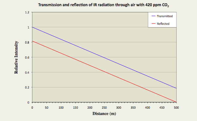
Fig. 92.1: The relative intensities of transmitted and reflected radiation in a 500 m long column of air with 420 ppm CO₂ that is heated equally from both ends. LT is radiation transmitted from left to right when the heating is at x = 0 m, and LR is the amount reflected. RT is radiation transmitted from right to left when the heating is at x = 500 m, and RR is the amount reflected.

In Fig. 92.1 the curve TL (blue curve) represents the radiation incident from the left at x = 0 m which is then partially reflected by the greenhouse gas to create a reflected flux RL (red curve) that propagates from right to left, building in strength as it propagates. This much is identical to the situation in Fig. 91.3 in the previous post. However, in the case of Fig. 92.1 an identical radiation flux RT also enters the column of gas from the right (green curve). This is also partially reflected by the greenhouse gas to create a reflected flux RR (violet curve) that propagates from left to right. The net result is that there are now two radiation fluxes travelling from left to right (TL and RR), and two travelling in the opposite direction (LR and RT). 

It can then be seen that the total radiation flowing from left to right will be the sum of LT and RR, which will be a constant value of 1.0 at all points along the gas column. The same is true for the total radiation flowing from right to left. In other words, the radiation that is emitted at the right hand exit of the column (x = 500 m) balances exactly the energy that entered initially at x = 0 m. Similarly the radiation that is emitted at the left hand exit of the column (x = 0 m) exactly balances the energy that initially entered at the right (at x = 500 m). This result leads to three important conclusions. 

The first is that in this situation the gas must be isothermal. This follows from the Schwarzschild's equation (see Eq. 91.6 in Post 91). As the total radiation flux in both directions is constant, it follows that the differentials of both I_u(x) and I_d(x) must be zero and so the following equality must hold at all points x.

I_u(x) = I_d(x) = B(λ,T)

(92.1)

As I_u(x) and I_d(x) are both independent of x, then it follows that B(λ,T) must be as well. In which case the temperature T must be independent of x.

The second is that the radiation emitted at each end of the column in not just the radiation that entered at the opposite end. Some of it is radiation that has been reflected by the greenhouse gases via the Greenhouse Effect. This is an important point that is lost on many. It is often falsely claimed that because the gas is isothermal and the radiation flux exiting the gas balances that entering at the opposite end, then this must mean that the Greenhouse Effect is not in operation. Actually it is. It just appears not to be.

The third conclusion is that the Beer-Lambert law cannot be valid in this situation as it cannot explain this result. If the transmitted radiation fluxes LT and RT obeyed the Beer-Lambert law then they would both decay exponentially with distance into the gas, and so too would their reflected fluxes LR and RR. This would mean that the total flux in each direction at the centre of the gas column would be less than at the ends. The laws of thermodynamics cannot allow this to happen as it would lead to a permanent temperature decrease from each end towards the centre. Energy would flow into the centre only to disappear there in violation of the law of conservation of energy. So the Beer-Lambert law is a red herring in this instance.

2) The Greenhouse Effect for Earth's atmosphere

The Earth's atmosphere deviates from the examples I have discussed so far in one major respect: its density, n(x), decreases with height, x. This density change is more or less exponential over most of the lowest 80 km and is of the form 

n(x) = n_o e^-kx

(92.2)

where k = 0.15 km^-1. As the relative concentration of carbon dioxide (CO₂)in the atmosphere is remarkably constant at about 420 ppm for all altitudes up to at least 80 km, it then follows that the CO₂ density will also decay with altitude, x, in accordance with Eq. 92.2 as well with n_o = 0.018 mol/m³. As the atmosphere is mainly heated from the bottom by the Earth's surface this decrease in density with height will significantly effect the nature of the Greenhouse Effect.

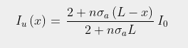
The strength of the Greenhouse Effect can be determined by substituting the expression for n(x) shown in Eq. 92.2 into Eq. 91.5 in Post 91. It is then possible to solve for I_u(x) subject to the constraint that the difference between I_u(x) and I_d(x) remains constant for all values of x due to conservation of energy as I explained in Post 88. The result is that I_u(x) varies with x as

(92.3)

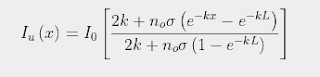
where σ is the absorption/emission cross-section of the CO₂ molecules and L is the total height of the atmosphere. It then follows (by setting x = L in Eq. 92.3) that the total amount of radiation emitted at the top of the atmosphere into outer space will be ΛI_o where the emitted fraction Λ is given by

 (92.4)

Subtracting ΛI_o from Eq. 92.3 then gives the associated expression for the downwelling radiation

(92.5)

As the height of the atmosphere, L,  exceeds 80 km, and k is much smaller than n_oσ, it can then be seen that Eq. 92.4 will approximate as

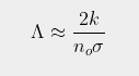
(92.6)

This is virtually identical to the result shown in Eq. 91.10 in Post 91, but with L replaced by 1/k. This is not very surprising as the mathematics of integral calculus tells us that 1/k is the effective thickness of an atmosphere that gets exponentially thinner with increasing height. It also indicates that the amount of radiation that escapes at the top of the atmosphere will decrease inversely (i.e. reciprocally) with CO₂ concentration and not exponentially as predicted by the Beer-Lambert law. This is shown graphically in Fig. 92.2 below where I_u(x) based on Eq. 92.3 at each altitude x is compared to the expected transmission based on the Beer-Lambert law. The difference is striking.

 

Fig. 92.2: A comparison of the amount of 15 µm IR radiation transmitted upwards at different heights in the atmosphere (blue curve) compared to that predicted by the Beer-Lambert law (red curve).

What Fig. 92.2 shows is that the amount of 15 µm radiation escaping at the top of the atmosphere is much greater than many people think. According to the Beer-Lambert law it should be so low as to be unmeasurable. In reality it could be as much as 1.5%. The blue curve in Fig. 92.2 does fall exponentially, but not to zero: it tends asymptotically to Λ. The value of Λ also depends on the nature of the atmosphere as Eq. 92.4 shows. However, its dependence on CO₂ concentration is reciprocal not exponential. This is why more radiation escapes than many people intuitively think can do.

Summary

The examples outlined in this post show that the Greenhouse Effect is more complex than the simplistic model that is generally presented. Even thick layers of greenhouse gas will emit appreciable amounts of infra-red radiation from within their absorption bands. Relying on the Beer-Lambert law will result in at best an incomplete picture, and at worst a totally misleading one.

Yes, the amount of IR radiation transmitted by the Earth's atmosphere reduces exponentially with height, at least at lower altitudes, but this is not due to its absorbing properties associated with the Beer-Lambert law. It is due primarily to the exponential drop in CO₂ concentration with height. Even then this exponential fall never tends to zero as Eq. 92.3 and Eq. 93.4 demonstrate, but instead tend to a finite transmission value Λ that could be as much as 1.5%.

91. The Schwarzschild equation and scattering

In Post 86 I showed how the Greenhouse Effect can be viewed as resulting from a combined process of absorption of infra-red radiation by molecules of carbon dioxide (CO₂), followed by re-emission of the same wavelength of radiation, but in a different random direction. The law that leads to this result is the principle of detailed balance. I also showed how this process resembled a scattering process, but with a much greater strength due to the significantly greater absorption cross-section (σ_a) of CO₂ compared to its cross-section for Rayleigh scattering, σ_s. Therefore it could be modelled as a scattering process, but one with an appropriately large cross-section.

Then in Post 88 I showed how this combined process of absorption and re-emission resulted in absorption that decreased linearly with distance x into a gas of uniform density, rather than exponentially as predicted by the Beer-Lambert law. The importance of this result is that it demonstrates that the transmission of radiation through an absorbing gas will be greater than that predicted by the Beer-Lambert law, and so changes to the concentration of the absorbing gas will have a larger impact on the overall transmission than the Beer-Lambert law would predict. 

Sadly this result has been questioned by some who have claimed that the scattering (or combined absorption and re-emission) approach is not valid as it does not follow from, or agree with, Schwarzschild's equation. This equation is possibly named after the German physicist Karl Schwarzschild (shown below), although it could actually be named after his son Martin Schwarzschild who worked in the field of stellar evolution. In this post I will show that this claim of non-validity is not true and that Schwarzschild's equation leads to the exact same results as I outlined in Post 88.

 Fig. 91.1: Karl Schwarzschild (1873-1916)

The Model

In order to understand the Greenhouse Effect we need to consider the radiation flows through a thin layer of gas of thickness δx at some altitude x, and then extend this to model to the gas as a whole. In particular, we need to consider radiation flows through the gas from opposing directions. This is because each thin layer of the gas only absorbs a small fraction of radiation passing through it. Most of the rest is then absorbed by subsequent layers above the initial layer. However, after absorption the radiation is re-emitted and the re-emission process occurs equally in both directions (up and down). This means that some of this emitted radiation will travel in a downwards direction and reheat the first layer from the opposite direction. This is why the Beer-Lambert law fails.

In order to model this process we need to consider radiation fluxes in both directions as shown in Fig. 91.2 below. Let's assume that the gas has a concentration or particle density n(x), and each molecule of it has an absorption cross-section σ_a. If radiation of intensity I_u(x) travels in an upward direction from a hot surface and enters the gas layer from below, as shown in Fig. 91.2 below, a proportion of it will be absorbed by the gas. This in turn will heat the gas and cause it to emit radiation in both an upwards and a downwards direction. The result will be that the intensity of upward radiation leaving the gas layer will change by an amount δI_u(x).

Fig. 91.2: A schematic illustration of how scattering, absorption and thermal emission within each thin layer of the atmosphere alters the intensities of the upwelling (I_u) and downwelling (I_d) radiation.

The upwelling radiation will then go on to interact with gas above the layer shown in Fig. 91.2 and thus heat this gas as well. This gas will then re-emit radiation, some of it in a downward direction, and this downwelling radiation I_d(x) will then also pass through our original layer of gas. It in turn will be partially absorbed, heating the gas and causing it to radiate. The net result is that the intensity of the downwelling radiation leaving the gas layer will also change, in this case by an amount δI_d(x). So far this model is identical to the one outlined in Post 88. The next step is to consider the changes of intensity, δI_u(x) and δI_d(x), using Schwarzschild's equation and the Planck function, B(λ,T), where λ is the wavelength of the radiation and T is the temperature of the gas in kelvins at this height x. In the following discussion I will consider the absorption and re-emission of radiation at a fixed wavelength λ.

The Proof

As the upwelling radiation I_u(x) at a fixed wavelength λ passes through the thin layer of gas of thickness δx a small amount of it will be absorbed by the gas. This amount will be proportional to the number of molecules encountered per unit area, n(x)δx, their absorption cross-section, σ_a, and the amount of radiation in the original flux, I_u(x). The result is that the transmitted intensity will decrease by an amount equal to I_u(x)σ_an(x)δx.

At the same time the thin layer of gas will be emitting radiation in both the upward and downward direction due to its temperature T. This temperature will in turn vary with height x, so both B(λ,T) and I_u(x) will vary with x. The intensity emitted in each direction is given by the Planck function, B(λ,T), multiplied by the number of molecules per unit area in the layer, n(x)δx, and the emission cross-section, σ_e. The result of this emission process is that the transmitted intensity above the layer will increase by an amount equal to B(λ,T)σ_en(x)δx.

Combining these two effects of emission and absorption gives the total change in intensity of the upwelling radiation

δI_u(x) = [B(λ,T)σ_e - I_u(x)σ_a]n(x)δx

(91.1)

This is Schwarzschild's equation. However, it is only half the solution because there is a similar equation that can be derived for the changes to the downwelling radiation I_d(x) in the thin layer at the same wavelength λ. Thus the resulting equation will be

δI_d(x) = [B(λ,T)σ_e - I_d(x)σ_a]n(x)δx

(91.2)

Finally, there is one other consideration we must take into account: energy conservation at wavelength λ. The total energy flowing into the layer of gas must match the energy flowing out. This means that 

δI_u(x) + δI_d(x) = 0

(91.3)

and so

[ I_u(x) + I_d(x) ]σ_a = 2B(λ,T)σ_e 

(91.4)

We can now eliminate B(λ,T)σ_e from Eq. 91.1 and Eq. 91.2 and turn both equations into first order differential equtions. However, because the change in downwelling radiation I_d(x) in Fig. 91.2 is defined to be positive for changes of x in a negative direction the δx term must be negative, and therefore the differential term dI_d/dx = - δI_d/δx.This means that

 (91.5)

It then turns out that Eq. 91.5 is identical to Eq. 88.5 in Post 88. So if the equations are the same and the boundary conditions are the same, then the solutions must be the same as in Post 88. So even using Schwarzschild's equation as our starting point we end up with the same result. 

Finally, we can write Schwarzschild's equation as two differential equations, one for I_u(x) and one for I_d(x). From Eq. 91.1 we get the obvious result

(91.6)

The equivalent equation for I_d(x) is similar, but requires some explanation.

(91.7)

In Eq. 91.7 the order of the I(x)σ_a and B(λ,T)σ_e terms to the right of the equality sign have been reversed compared to Eq. 91.6. This is because the downwelling radiation, I_d(x), is flowing in the negative direction through the thin gas layer. So for I_u(x) the radiation term B(λ,T)σ_e is directed in the same direction as I_u(x) so it must be positive, while the absorption in the gas layer must leads to a lower value of I_u(x) above the layer than below. In the case of I_d(x) the reverse it true in both cases, hence the reversal of sign for both terms.

Finally, it should be noted that conditions of thermal equilibrium generally require the cross-sections σ_a and σ_e to be equal. This is particularly true for black body radiation where a black body at constant temperature must emit what it absorbs, otherwise it will gain or lose energy, and thus not be at constant temperature.

 

Implications

If we now apply the above results to a real system and consider the case of a column of gas of thickness L, and uniform density n that is independent of x, the model outlined above means that the upwelling radiation will vary with x through the gas as (see Post 88)

(91.8)

where I_o is the intensity of radiation entering the gas at x = 0, while the downwelling radiation will vary as

(91.9)

The difference between I_u(x) and I_d(x) will be constant (ΛI_o), as required by energy conservation, and will be equal to the amount transmitted at the end of the column (i.e. at x = L), so 

(91.10)

In Fig. 91.3 below I have suggested what I_u(x) and I_d(x) might look like through a 500 metre long horizontal column of air with 420 ppm of CO₂ when it is irradiated with 15 µm infra-red radiation from one end. It should be noted, though, that this theoretical data is based on an estimated value for the scattering cross-section of the CO₂ molecules that could be almost a factor of ten too small. Nevertheless, it still illustrates qualitatively how the transmission of 15µm infra-red radiation changes through the gas, and also how the Greenhouse Effect (as defined by the relative intensity of the reflected radiation at x = 0) is related to this transmission (see the red curve in Fig. 91.3).

Fig. 91.3: The relative intensities of transmitted (I_u) and reflected (I_d) radiation along a 500 metre column of air containing 420 ppm of CO₂ with an absorption cross-section of 1.6 x 10^-24 m².

The graph in Fig. 91.3 suggests that a 500 metre column of air will transmit less than 18% of the incident radiation and reflect back the rest. The question is: is this more or less than that predicted by the Beer-Lambert law? The answer to this can be seen in Fig. 91.4 below.

Fig. 91.4: The relative intensities of radiation transmitted  through a column of air of length L containing 420 ppm of CO₂ with an absorption cross-section of 1.6 x 10^-24 m² based on two different models: (i) a backscattering model described by Eq. 91.10 (blue curve), and (ii) the Beer-Lambert law (red curve).

The blue curve in Fig. 91.4 demonstrates how the transmission through a column of air would decrease with the length of the column, L, if half of the absorbed radiation is backscattered or re-emitted in the reverse direction and half is re-emitted in the forward direction. The result is a curve that decays with L in accordance with Eq. 91.10. The red curve on the other hand shows how the transmission would change if it followed the (commonly accepted) Beer-Lambert law where the transmitted intensity varies with L as

(91.11)

What is clear is that the Beer-Lambert law underestimates the transmission for large values of L, and in effect predicts that there is no significant transmission beyond 400 metres. The blue curve shows that this is not the case with over 10% transmission for a column of length 1000 metres. In practice this means that the Beer-Lambert law will massively underestimate the impact of future increases in CO₂ levels because it will assume that the backscattering is already operating at close to 100% or saturation with 420 ppm of CO₂. Yet clearly it is not. In fact even at 10 km (the effective thickness of Earth's atmosphere) there is still more than 1% transmission. While this is small, it is not insignificant, particularly when considering the relatively small changes to the overall size of the Greenhouse Effect that are needed to create a warming of 1.5°C.

Caveats

The only condition I have applied to the proof and discussion described here is that set out in Eq. 91.4, which basically demands that each layer of the gas radiates the same amount of energy at each wavelength as it absorbs from the two fluxes, I_u(x) and I_d(x). This will be true provided all the heat of wavelength λ entering the gas originates from the Earth's surface at the bottom of Fig. 91.2, or at the very top of the atmosphere. In which case, the exact functional forms of I_u(x) and I_d(x) will depend only on the functional form of n(x) and the boundary conditions. However, at the top of the atmosphere this condition will not be satisfied as some of the incoming ultraviolet radiation from the Sun is absorbed there before it reaches the ground and so gets converted to infra-red radiation within the upper atmosphere. This means that Eq. 91.4 is no longer satisfied for each and every infra-red wavelength of interest within the gas.

In my next blog post I will consider a number of distinct and important examples to demonstrate how dependent the transmission is on the density profile of the gas, n(x), and also on the location of the heat source(s). These examples will also show that even when it sometimes looks like there is no Greenhouse Effect in operation, it is still there.

90. Lateral thought #5: Without fossil fuels there would be no Champagne

 

Yes, amazing as it seems, without coal we might not have Champagne. Well, possibly.

This tale arises out of the English energy crisis in the early 17th century (see here). After over one hundred years of shipbuilding for the new Royal Navy the country ran out of wood. There were of course other reasons such as population growth and increased urbanization that were equally to blame, just as they are today. But the net result was there were just not enough trees. So much for renewable energy.

In response a worried King James I banned the use of wood for non-essential purposes. And one of the areas to feel the heat was glass-making. In response they switched to using coal, which had previously been considered a dirty and ungodly fuel even though it was abundant. Yet needs must when the Devil drives. And there was an unexpected bonus, as there often is when the Devil is in play. By using coal English glass-makers were able to achieve higher kiln temperatures. This meant they could make glass bottles that were thicker and stronger - just what you need to make Champagne. Otherwise the bottles have a tendency to explode.

So, three cheers for fossil fuels. And yet another reason why the French love the English.

Of course this does raise an important philosophical question. Can you be a Champagne socialist and still fight for climate justice? I don't know. And until I do I'll probably stick to the Château Haut-Brion.